Assignment 8
1 General information
The exercises here refer to the lecture 8-9/BDA chapter 7 content.
The exercises constitute 96% of the Quiz 8 grade.
We prepared a quarto notebook specific to this assignment to help you get started. You still need to fill in your answers on Mycourses! You can inspect this and future templates
- as a rendered html file (to access the qmd file click the “</> Code” button at the top right hand corner of the template)
- Questions below are exact copies of the text found in the MyCourses quiz and should serve as a notebook where you can store notes and code.
- We recommend opening these notebooks in the Aalto JupyterHub, see how to use R and RStudio remotely.
- For inspiration for code, have a look at the BDA R Demos and the specific Assignment code notebooks
- Recommended additional self study exercises for each chapter in BDA3 are listed in the course web page. These will help to gain deeper understanding of the topic.
- Common questions and answers regarding installation and technical problems can be found in Frequently Asked Questions (FAQ).
- Deadlines for all assignments can be found on the course web page and in MyCourses.
- You are allowed to discuss assignments with your friends, but it is not allowed to copy solutions directly from other students or from internet.
- Do not share your answers publicly.
- Do not copy answers from the internet or from previous years. We compare the answers to the answers from previous years and to the answers from other students this year.
- Use of AI is allowed on the course, but the most of the work needs to by the student, and you need to report whether you used AI and in which way you used them (See points 5 and 6 in Aalto guidelines for use of AI in teaching).
- All suspected plagiarism will be reported and investigated. See more about the Aalto University Code of Academic Integrity and Handling Violations Thereof.
- If you have any suggestions or improvements to the course material, please post in the course chat feedback channel, create an issue, or submit a pull request to the public repository!
- The decimal separator throughout the whole course is a dot, “.” (Follows English language convention). Please be aware that MyCourses will not accept numerical value answers with “,” as a decimal separator
- Unless stated otherwise: if the question instructions ask for reporting of numerical values in terms of the ith decimal digit, round to the ith decimal digit. For example, 0.0075 for two decimal digits should be reported as 0.01. More on this in Assignment 4.
1.1 Assignment questions
For convenience the assignment questions are copied below. Answer the questions in MyCourses.
Lecture 8-9/Chapter 7 of BDA Quiz (96% of grade)
This week’s assignment focuses on hierarchical models and modelling with brms.
1. ELPD
In order to evaluate a model, for comparison to other models or for model checking purposes, it is useful to measure how well predictions match the data. Preferably, the measure of predictive accuracy is tailored to the data-application (application specific cost-function or decision theoretic quantity, discussed more next week). But in the absence of that, we might choose from a range of scoring functions or rules mentioned in the lecture/book (see for more details on general scoring functions or rules in Gneiting and Raftery (2007)). For the below denote the target as \(y\) and potential covariates as \(x\).
1.1 Which expression below defines the log-score for observation \(y_i\)?
1.2 Why is the log-score a convenient scoring rule?
1.3 Denote by \(\tilde{y}\) unseen target data with distribution \(p_t(\tilde{y})\) and by \(y\) target data that is conditioned on for posterior inference on model parameters. Which of the following refers to the expected log-predictive density for new data points \(\tilde{y}_1\dotsc,\tilde{y}_n\)?
1.4 Suppose \(\tilde{y} = y\), then elpd reduces to the log point-wise predictive densities (lpd) for observations \(y_1,\dotsc,y_n\). Why is lpd often a bad estimate for elpd?
1.5 We often use leave-one-out cross-validation (LOO-CV) to approximate out-of-sample performance. Denote by \(y_{−i}\) all but the ith observation for \(y\) and by \(\int p(y_i\mid\theta)\,p(\theta\mid y_{-i})\,\mathrm{d}\theta\) the posterior predictive distribution for the ith data point based on data leaving out the ith data point. Which of the expressions below refers to the Bayesian LOO-CV estimate of the out-of-sample predictive fit \(\mathrm{elpd}_{\mathrm{LOO}}\)?
1.6 Instead of computing the LOO predictive densities n times for n left-out observations, a computationally much more efficient approach is to fit the model once and use importance sampling to approximate the n LOO densities in \(\mathrm{elpd}_{\mathrm{LOO}}\). Which of the below refers to the importance sampling estimate of \(\mathrm{elpd}_{\mathrm{LOO}}\)? Assume \(\sum^S_{r=1}\tilde{w}_i^{(r)}=1\) for all \(i\).
1.7 Use \(p(\theta \mid x,y)\) as the proposal distribution for \(p(\theta \mid x_{−i},y_{−i})\). Derive the expression for the unnormalised importance weights \(w^{(s)}i\) (up to a constant of proportionality), assuming that the likelihood conditional on \(x\) and \(y\) can be factorised by \(i=1,\dotsc,n\). Which of the below is proportional to the desired importance weight draw for the \(s\)-th draw of the posterior and observation \(i\)?
1.8 Derive the expression for the self-normalised importance sampling estimator with the weights derived in 1.7. Which of the below is correct?
The importance sampling estimator can also be extended to other scoring functions/rules. In particular, it will be of advantage for the projects to review the \(R^2\) (coefficients of determination), Root-mean-squared-error (RMSE) which measure relative variance fit and point predictive accuracy respectively, as well as the Probability Integral Transform (PIT), and their associated cross-validated variants. These are easily implemented with BRMS fit objects. See the BRMS manual as well as the Bayes \(R^2\) case study further details on implementation for some of these.
ELPD assesses predictions in terms of the sharpness (concentration) (for log-score this is related to negative entropy), as well as calibration (coverage) of the predictive distribution. Sharpness of the predictive distribution is rewarded since narrow predictive distributions have higher densities. On the other hand, too narrow distributions have high density in too narrow region, and lower density elsewhere. The probability intervals (e.g. central intervals) cumulative density functions of a calibrated distribution match the distribution of the target. It is possible that two different models are both well calibrated, but they have different sharpness, for example, if one of the models has additional covariate which helps to reduce the predictive uncertainty. In the below we will further discuss how to visually assess calibration. This belongs to the posterior predictive checks discussed during the lecture, and are useful to check first before formally evaluating models with ELPD (and other scoring functions/rules).
1.9 We can measure calibration by transforming the comparison between an observation and the conditional predictive distribution to a value between \([0,1]\). Define \(y^{\mathrm{rep}}_i\) as a draw from the predictive distribution \(p(\tilde{y}_i\mid y_i)\), which transformation should we use?
1.10 This transformation is called the probability integral transform (PIT). How should the PITs be distributed with infinite data, if the predictive distribution is correctly calibrated?
When dealing with finite data, we can only hope to be close enough to uniform
and you can use the ppc_loo_pit_overlay() function from bayesplot
to visually check for the posterior uncertainty in the (cross-validated) PIT
values.
Instead of looking at the distribution of PIT values, it can be easier to examine the cumulative distribution function of the PIT values, which should be close to a 45-degree line, since the large sample distribution is uniform. The below is taken from the BRMS demo 13.
Suppose the kernel density estimates of the predictive distribution and data look the following:
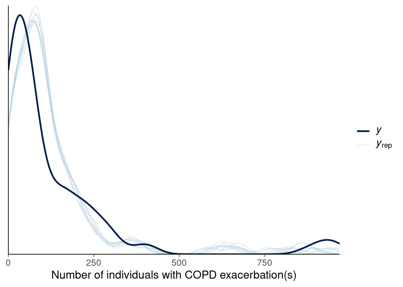
Figure 1
1.11 What can you say about calibration from this model for the data?
1.12 Based on the model in Figure 1, which of the plots below match the ECDF plot (light blue envelope indicates regions of acceptable ECDF values)?
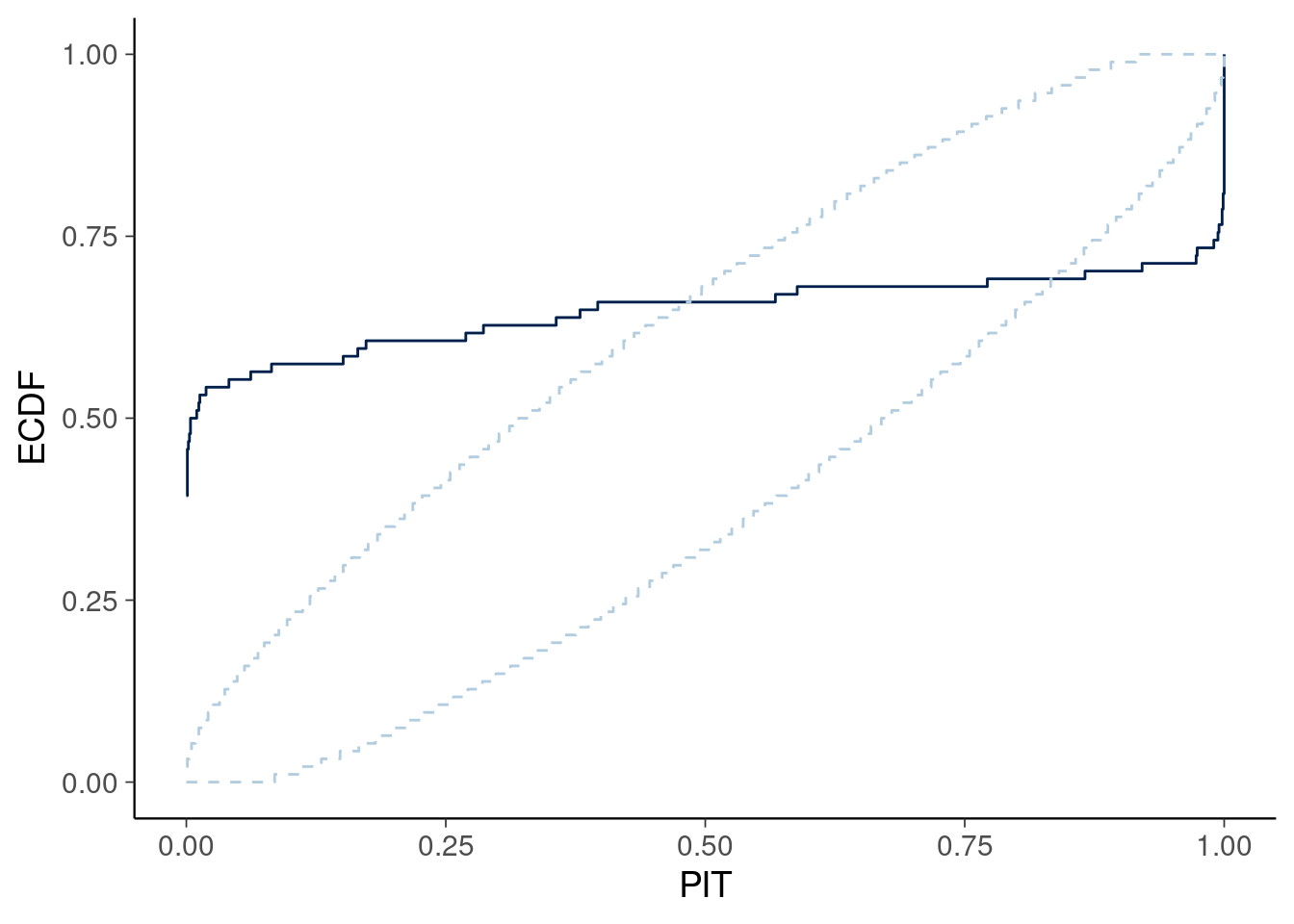
Figure 2
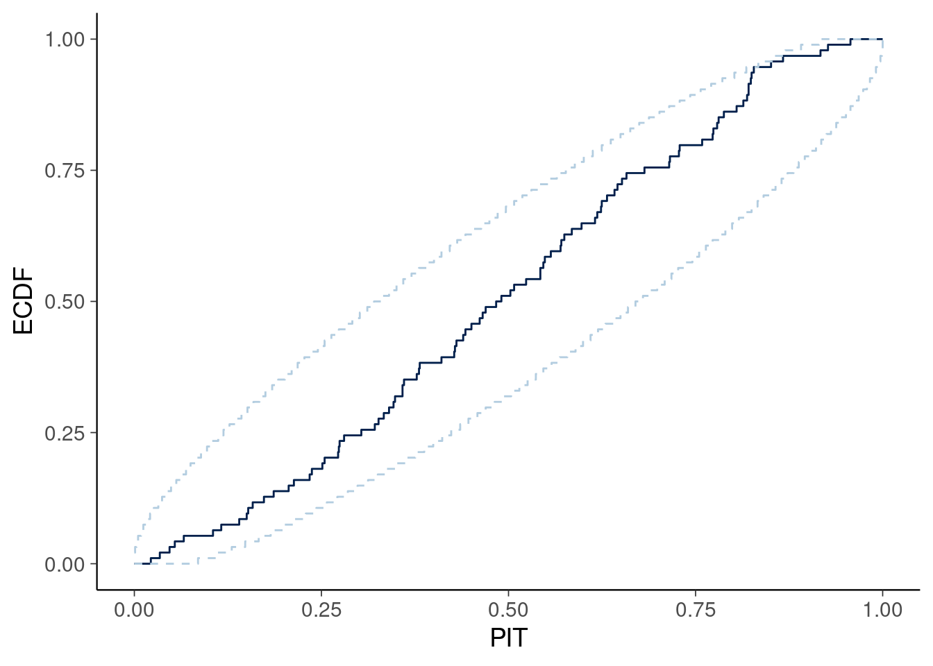
Figure 3
Suppose the revised model produces the following predictive distribution:
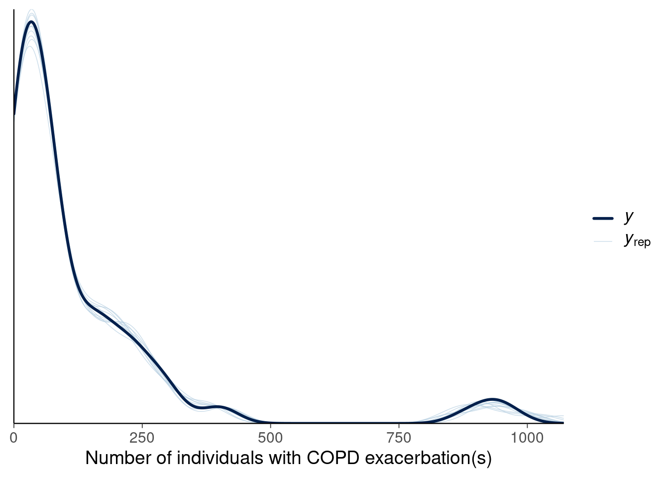
Figure 4
1.14 Based on the model in Figure 4, which of the plots below match the ECDF plot (light blue envelope indicates regions of acceptable ECDF values)?
Figure 5
Figure 6
2.2 Assuming that importance weights have finite variance and mean, we can use the standard CLT to guarantee variance reduction at rate 1/S, where S is the number of MCMC draws. Different CLTs can be applied depending on the existence of certain fractional moments (fractional moments are more general than integer moments and are useful in describing properties of fat-tailed distributions). To estimate the number of fractional moments of the weights, we can model the tails of the importance weights using insights of extreme value theory (Pickands, 1975). What distribution can be used to estimate the number of fractional moments?
We refer to the estimated value of 1/k as the k-hat value reported as a diagnostic in the loo package. Since most distributions have tails that are well approximated by GDP, we can replace tail weights of the importance weight distribution with the expected ordered statistics of the fitted GDP. In the context of LOO, we refer to this as Pareto smoothed importance sampling (PSIS-LOO).
2.3 What is the rationale of replacing largest weights by the expected ordered statistics of the fitted GDP?
2.4 Based on the above, suppose importance weights follow a standard Cauchy distribution. What k-hat value do you expect with sufficiently large number of draws?
2.7 What are common causes for large k-hats within the context of PSIS loo?
2.8 What should you consider doing if you have high k-hat values?
3. Sleep study
In Assignment 7, you fit two different models to the sleepstudy dataset. One with varying intercepts per person and one with varying intercepts and slopes. In this exercise you will perform visual checks and leave-one-out cross-validation on these models.
First, perform the following steps for the varying intercept model. This model allows for different Subjects to have different baseline Reaction times (before sleep deprivation).
Use pp_check(fit) to create the default density overlay plot.
3.1 Which of the following best describes the interpretation of the plot?
Next try a different plot of the predictions: pp_check(fit, type =
"intervals_grouped", x = "Days", group = "Subject")
3.2 What does the plot present?
3.3 Based on the plot, what can you say about how the model predicts the observations of individual Subjects?
Next, use PSIS-LOO CV to estimate the elpd of the varying intercepts model.
3.4 The elpd_loo estimate for the varying intercepts model is and the standard error estimate is .
The second model estimates varying intercepts and varying slopes. This model allows for different effects of Days for each Subject.
Plot again the default density plot of predictions using
pp_check()
3.5 Which best describes the plot:
Perform PSIS-LOO CV to estimate elpd_loo for the varying intercepts and slopes model. You may find that there are high Pareto-k values. These can be fixed with importance weighted moment matching at the cost of some computation, but in this case the elpd_loo will change negligibly with the improved estimates.
3.6 The elpd_loo estimate for the varying slopes and intercepts model is and the standard error estimate is .
So far you have only performed visual posterior checks to compare the models.
However, another option is to compare the leave-one-out cross validation
values between the models. Use loo_compare() to calculate the
elpd_diff between the two models.
3.7 The elpd_diff estimate is (enter as negative value as shown in the loo_compare output) and the standard error is .
3.8: Which of these best describes the conclusions from the loo comparison:
4. Sleep study extensions
So far you only compared the two models that were fit in the previous week. But modelling is an iterative process, and additional features of the data can be modelled. Next, you will add three extensions to the previous models, which you may have thought about already: (1) Reaction times are known to be positively skewed (2) There could be a non-linear relationship between Days and Reaction time (3) As seen in the previous assignment, there are likely some outliers for some groups.
The first issue can be tackled by changing the observation family to a positively skewed distribution, such as log-normal. As this transforms the interpretation of the coefficients, the priors should be updated. Use the following priors with the lognormal observation family:
\(\alpha_0 \sim \mathrm{normal}(\log(250),1)\)
\(\beta_0\sim \mathrm{normal}(0,1)\)
\(\sigma\sim\mathrm{normal}(0,2)\)
\(\alpha_j\sim\mathrm{normal}(0,\tau_{\alpha})\)
\(\beta_j\sim\mathrm{normal}(0,\tau_{\beta})\)
\(\tau_{\alpha}\sim\mathrm{normal}(0,1)\)
\(\tau_{\beta}\sim\mathrm{normal}(0,1)\)
Fit the varying slopes and intercept model with lognormal family.
4.1 Plot the default pp_check(). What do you
notice?
Estimate the elpd_loo for the lognormal model.
4.2 The elpd_loo estimate for the lognormal model is , and the standard error estimate is .
4.3 How does this compare to the other models with respect to LOO-CV?
Next, to address potential non-linear effect with respect to Days, you can
try with a spline term for Days. This allows for a non-linear population-level
effect of Days on Reaction time. Add the term s(Days) to the
formula for the lognormal model, and compare to the other models using
pp_check and loo_compare. Use a normal(0, 1) prior on the sDays_1
term.
4.4 Based on elpd_loo comparison:
4.5 To make inference robust to outliers, we could instead
change the observation model to the student-t. Keep s(Days) in
the model without specifying a prior for sDays_1 (the default is
a student_t prior in brms and in this case good enough) as well as the varying
intercept and slope. Use the default prior (gamma(2,0.1)) in brms
for the degrees of freedom. Do you find evidence for fat-tails? What is the
posterior estimate of the degrees of freedom parameter \(\nu\)?
4.6 The elpd_loo estimate of the student-t model is:
4.7 Plot the conditional_effect() (as in
Assigment 7) for the student-t model. What do you observe in comparison to the
normal conditional effects?
4.8 Based on elpd_loo, the order of the 5 models from best to worst predictive performance is: