Assignment 9

Author

Aki Vehtari et al.

1 General information

The exercises here refer to the lecture 9-10 and BDA3 Chapter 9 content.

The exercises constitute 96% of the Quiz 9 grade.

We prepared a quarto notebook specific to this assignment to help you get started. You still need to fill in your answers on Mycourses! You can inspect this and future templates

as a rendered html file (to access the qmd file click the “</> Code” button at the top right hand corner of the template)

General Instructions for Answering the Assignment Questions

Questions below are exact copies of the text found in the MyCourses quiz and should serve as a notebook where you can store notes and code.
We recommend opening these notebooks in the Aalto JupyterHub, see how to use R and RStudio remotely.
For inspiration for code, have a look at the BDA R Demos and the specific Assignment code notebooks
Recommended additional self study exercises for each chapter in BDA3 are listed in the course web page. These will help to gain deeper understanding of the topic.
Common questions and answers regarding installation and technical problems can be found in Frequently Asked Questions (FAQ).
Deadlines for all assignments can be found on the course web page and in MyCourses.
You are allowed to discuss assignments with your friends, but it is not allowed to copy solutions directly from other students or from internet.
Do not share your answers publicly.
Do not copy answers from the internet or from previous years. We compare the answers to the answers from previous years and to the answers from other students this year.
Use of AI is allowed on the course, but the most of the work needs to by the student, and you need to report whether you used AI and in which way you used them (See points 5 and 6 in Aalto guidelines for use of AI in teaching).
All suspected plagiarism will be reported and investigated. See more about the Aalto University Code of Academic Integrity and Handling Violations Thereof.
If you have any suggestions or improvements to the course material, please post in the course chat feedback channel, create an issue, or submit a pull request to the public repository!

1.1 Assignment questions

For convenience the assignment questions are copied below. Answer the questions in MyCourses.

Lecture 9-10/Chapter 9 of BDA Quiz (96% of grade)

1. \( R^2 \) Prior

The coefficient of determination, \( R^2 \), measures the proportion of variance explained by the model compared to the total variance of the model. This metric can be easily extended to a Bayesian definition. Let \( \tilde{y} \) denote future data. Suppose a model uses covariates X to model the target y with parameters \( \theta \). Define \( \mu_n = E[\tilde{y}_n |X_n,\theta] \) as the expected predictor for future observations for all n and \( \epsilon_n = \tilde{y}_n - \mu_n \) as the modeled residual.

1.1: While for certain priors the implied probability distribution for Bayes \( R^2 \) may be derived analytically, we can generally find the push-forward distribution with Monte-Carlo Integration. Which of the below correctly characterises the s-th draw from the Bayes \(R^2\) distribution?

1.2 What is the intuition behind the Bayesian \(R^2\)?

1.3: Assume a normal observation model with variance \(\sigma^2\) and the predictor terms includes covariates X and coefficients \( \beta \). Which of the below is the correct expression for a draw from the Bayes-\(R^2\) distribution?

1.4: With some further assumptions, we can formulate Bayes-\( R^2 \) similarly for other observation families. For logistic regression, define \( \mu_n^{(s)} = logit^{-1}(X_n^T\beta^{(s)}) = \pi_n^{(s)} \) and \( E[var( \epsilon_n^{(s)}) | \theta^{(s)}] = \pi_n^{(s)}(1-\pi_n^{(s)}) \). Which of the below is the correct expression for a draw from the Bayes-\(R^2\) distribution?

For other GLMs, it is not so straighforward to define the Bayes-\( R^2 \), so in this course, we recommend showing the Bayes-\( R^2 \) only for normal and logistic regression models.

The prior-predictive distribution of \(R^2\) is also useful to look at in order to understand the impact of the prior choices on the expected amount of variance fit. For the below, assume \( y_i \sim normal(\beta^TX_i,\sigma) \). Assume the covariates, \(X \in \mathbb{R}^{N \times p} \), have been scaled to have 0 mean and variance 1, and p = 26.

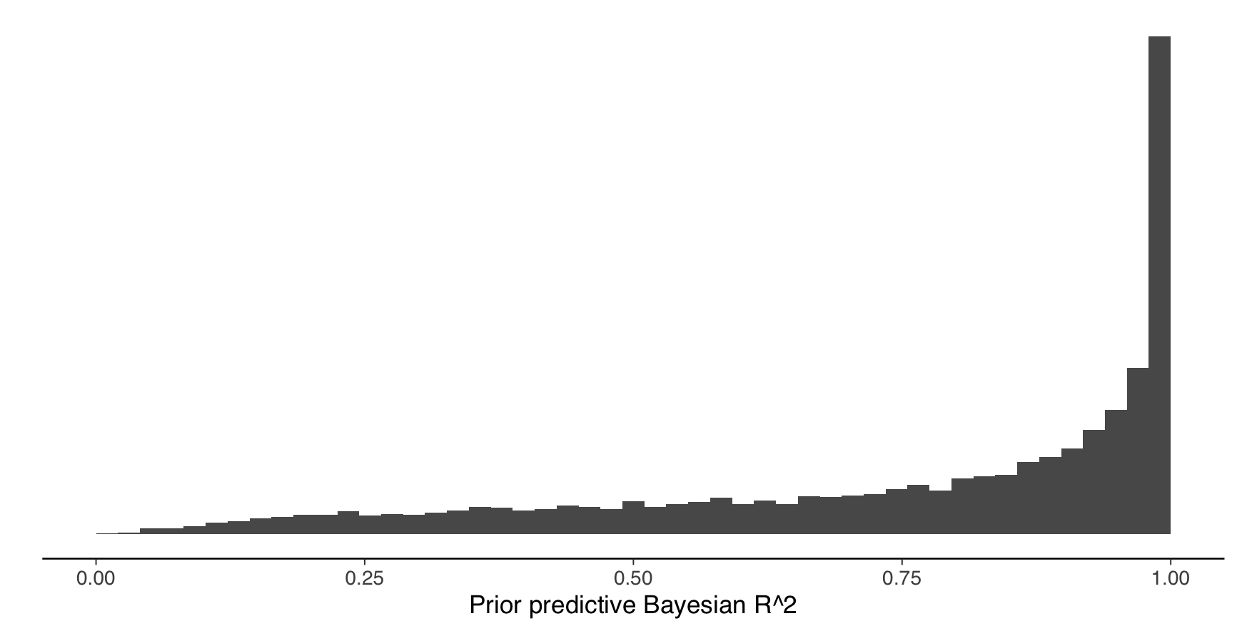
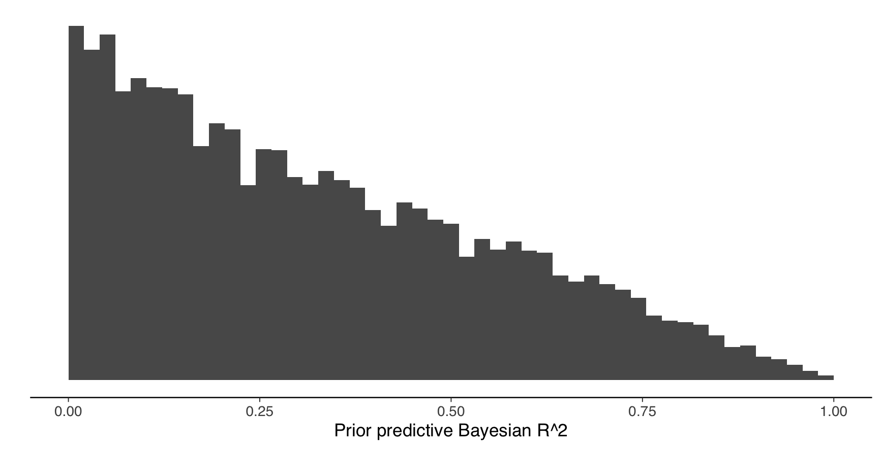
1.5: Assume standard normal priors for \(\beta\) and an exponential prior with rate 1/3 for \(\sigma\). Draw from the priors 4000 times, and generate prior predictive values for Bayes-\(R^2\). Which of the figures below refers to the correct implied \(R^2\) distribution?

1.6: With these priors you can derive the variance of the predictor term. What is the standard deviation of the predictor term?

You may also put a prior directly on the Bayesian-\( R^2 \). This is simplest for the normal linear regression model and implies a joint prior for \( (\beta,\sigma) \), where we specify beliefs about the \( R^2 \) and learn the rest of the hyper-parameters in the prior for \( \beta \) via partial pooling. In the prior hierarchy below, the beta distribution is parameterised in terms of a location \( \mu_{R^2}\) and scale \( \sigma_{R^2} \), where the relationship to the usual parameterisation of the \(beta (\alpha,\beta)\) distribution is \( \alpha = \mu_{R^2}\sigma_{R^2}, \beta = (1-\mu_{R^2})\sigma_{R^2} \):

\( \beta_j \sim normal(0, \sqrt(\tau^2\psi_j\sigma^2)) \)
\( \tau^2 = R^2/(1-R^2) \)
\( R^2 \sim beta(\mu_{R^2},\sigma_{R^2}) \)
\( \psi \sim Dir(\xi) \)
\( \sigma \sim \pi() \) (some distribution)

Here, we use the relationship between the variance of the predictor term \( X\beta \) and \(R^2\) to relate inference on the \( R^2 \) space to the population variance of \( \beta \), \(\tau^2\). If you are curious about this relationship, Zhang et al. (2022) provide derivations. \( \tau^2 \) is the population variance for the coefficients \( \beta \), which is allocated to individual coefficients via a weight vector \( \psi \). Positivity of weights \( \psi \) and sum to 1 constraint are enforced by assuming a Dirichlet distribution as prior. You may interpret \( \psi \) as determining the importance of a variable in explaining the variance of the target data, \(y\) (larger \( \psi_j \) compared to \( \psi_{-j} \) means that the j-th coefficient has larger variance and thus the j-th covariate contributes relatively more to the fraction of variance explained, \( R^2 \) ). The concentrations of the Dirichlet distribution, \( \xi \) can be used to encode prior information about the relative importance of covariates in terms of the fraction of variance explained. In absence of such prior knowledge, which is likely your starting point of your analysis, you may set these concentrations to 1. This implies that you think the covariates have equal importance. If you want to enforce sparsity on the coefficient vector, try setting to \( \xi = 0.3 \) (this pushes weights to the edges of the p-dimensional simplex)

1.8: Assume that \( \sigma \sim exp(1/3) \), \( \mu_{R^2} = 1/3, \sigma_{R^2} = 3 \) and \( \xi_j = 1 \) for all j in 1 to p. Which of the below distributions should the prior predictive Bayes-\(R^2\) be closest to? Assume the beta distributions below are parameterised in terms of location and scale.

1.9: Generate the prior predictive Bayes-\(R^2\) using the \(R^2 \) prior in 1.8 and and exponential prior with rate 1/3 for \(\sigma\). Draw from the priors 4000 times, and generate prior predictive values for Bayes-\(R^2\). Which of the figures below refers to the correct implied \(R^2\) distribution?

We generally recommend setting the prior for the \( R^2 \) with \( \mu_{R^2} = 1/3, \sigma_{R^2} = 3 \). This is weakly informative toward lower \( R^2 \) which may help regularising the coefficients' posterior variance, particularly in higher dimensions. You may experiment in your projects with those hyper-parameters in order to gauge sensitivity.

BRMS has the R2 prior implemented, and here some cautionary notes:

The implementation of the prior BRMS assumes you have scaled the covariates to have variance 1, so please pass scaled covariates to the brm function (the target variable should stay as is for easier model comparison).
The connection between R2 prior and model R2 is only exact for the normal model
We still recommend using the R2 prior in BRMS for all observation families, particularly when you have many covariates and you would otherwise use normal independent priors

For those who want to dig deeper, how would the prior for \( \beta \) need to be adjusted so that the \( R^2 \) of the model is invariant to changes in the scale of X?

2.Portuguese Student Data

Now we apply these priors to a data set in which the goal is to predict Portoguese students' final period math grade based on a moderately large set of covariates (p = 26), including social background and past schooling information.

Use the data preparation steps in the code template, and estimate a model with normal(0,1) priors on the regression coefficients, and otherwise use default priors.

2.1: Plot the marginal posteriors of the coefficients with this prior, what do you observe?

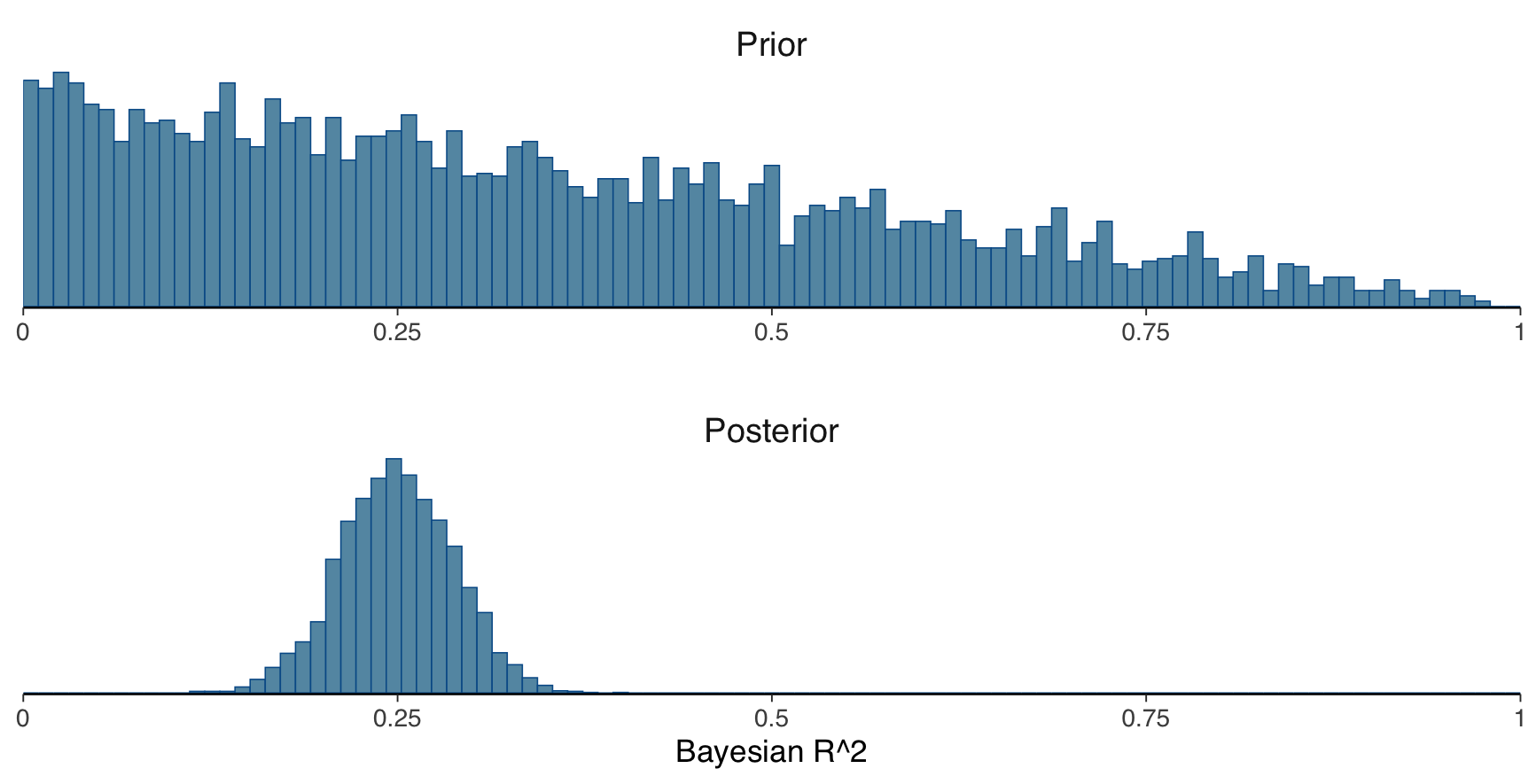
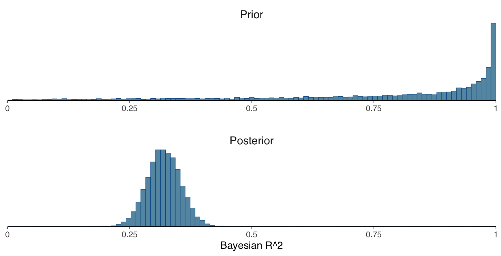
2.2: Compute and plot the prior and posterior Bayes-\(R^2\) distributions. Which of the figures below refers to the correct the implied \(R^2\) distribution with normal(0,1) priors on the regression coefficients?

2.3: Compute the mean of the posterior R2 distribution and the mean of the loo R2 .

2.4: What does the difference between the mean of the posterior R2 and LOO cross-validated R2 distribution indicate?

2.5: Now use the \( R^2 \) prior with \( \mu_{R^2} = 1/3, \sigma_{R^2} = 3 \) and concentration values of 1, otherwise use default priors from BRMS. Plot the marginal posteriors of the coefficients with this prior, what do you observe compared to the marginal posteriors of the normal(0,1) prior?

2.6: Compute and plot the prior and posterior Bayes-\(R^2\) distributions. Which of the figures below refers to the correct the implied \(R^2\) distribution using the \( R^2 \) prior ?

2.7: Compute the mean of the posterior predictive R2 distribution and the mean of the loo R2 .

2.8: What does the difference between the mean of the posterior R2 and LOO cross-validated R2 distribution indicate?

3. Bayesian Decision theory

3.1 Which of the following are steps of decision analysis according to BDA3?

4. Decision theory case study

Assume we created a model that estimates life expectancy of a person based on various covariates such as gender, history of diseases and so on. We conducted inference in a Bayesian way by obtaining samples of the parameters of our model.

A 80-year-old man with an apparently malignant tumor in the lung must decide between the three options of radiotherapy, surgery, or no treatment. He visits us and asks to use our model to help him with his decision. A priori doctors told the man that there is a 80% chance that the tumor is malignant. By using our marvellous model, we sampled posterior predictive draws (ppd) for all cases which are interesting for us. To keep things simpler, we have obtained only 5 posterior draws from the distribution of the predicted remaining lifetime.

if the man has lung cancer and radiotherapy is performed, ppd of his life expectancy are: [4.4, 5.3, 5.1, 3.2, 4.9]
if the man has lung cancer and surgery is done, which is dangerous for this age and doctors give 30% chance of mortality, ppd of his life expectancy in a case of successful surgery are: [5.9, 6.3, 6.2, 5.7, 7]
if the man has lung cancer and no treatment is given, ppd of his life expectancy are: [1.1, 0.7, 0.9, 1.7, 0.4]
if the man does not have lung cancer (no malignant tumor), ppd of his life expectancy are: [6.8, 5.5, 8.8, 7.4, 9]. Assume also that if man is healthy, radiotherapy or successful surgery do not affect his life expectancy, however he still has 30% of dying during the surgery

We shall determine the decision that maximizes patient’s life expectancy. Compute expected life expectancy for the above cases using posterior predictive draws and given probabilities:

4.1: man does not have lung cancer (no malignant tumor) and no treatment is given or radiotherapy is performed:

4.2: man does not have lung cancer (no malignant tumor) and surgery is done:

4.3: man has lung cancer and performs radiotherapy:

4.4: man has lung cancer and surgery is done:

4.5: man has lung cancer and no treatment is given:

Then, using these quantities, compute expected life expectancy under each treatment (you should use information that there is 20% chance that the man does not have lung cancer (no malignant tumor)):

4.6: with radiotherapy:

4.7: with surgery:

4.8: with no treatment:

4.9: What should the man choose to maximize his expected life expectancy?