Assignment instructions
1 Introduction
In addition to R-markdown, Quarto can be used to write the assignment reports. This template contains essentially the same information as the old R-markdown template but we illustrate how you can use Quarto for the assignments.
Some useful resources to get started with Quarto (also an example of a list):
- Getting started with Quarto and Rstudio from the official webpage
- A comprehensive user guide from the official webpage
- Markdown basics
- Quarto FAQ for R-markdown users
- Awesome Quarto - list by Mickaël Canouil
The assignment needs to be completed on MyCourses where it appears in quiz style. However, to aid your learning, we recommend creating your assignment with assignment-specific templates (recommended, see e.g. the links at the top of assignment 1) where we give hints and some initial structures to answer code.
As with R-markdown, you can use the text editor of your choice, but RStudio’s editor is probably the easiest and you can choose the formatting (e.g. section headings, bolding, lists, figures, etc.) from the toolbar. Switching between the source and visual mode allows the quick preview of your formatting.
Note Aalto JupyterHub has everything installed and you should be able to render the templates to pdf without any further set-up, but if there are problems contact the TAs or get more information on this from the Quarto documentation. Alternatively, if you have problem with creating a PDF file, start by creating an HTML file and the just print the HTML to a PDF. You may also use other software to create the report PDF, but follow the general instructions in this file (see the pdf version of the template file).
2 Loaded packages
Below are examples of how to load packages that are used in the assignment. After installing the aaltobda package (this is pre-installed in Aalto JupyterHub), you need to also load it in the beginning of every notebook where you want to use it with library() function (also in Aalto JupyterHub):
3 Including source code
In general, all code needed to produce the essential parts is recommended to be included, so that it is possible to see, for peer reviewers (and TAs), where errors may have happened.
You can always look at the open rubrics to see how and what is asked for in each exercise.
Try to avoid printing an excessive amount of code and think about what is essential for showing how did you get the result.
Write clear code. The code is also part of your report and clarity of the report affects your score. If the code is not self-explanatory, add comments. In a notebook, you can interleave explaining text and code.
If in doubt additional source code can be included in an appendix.
4 Format instructions
All exercises in the assignment should start with a header fully specifying that it is exercise X, e.g.: (use # in quarto / rmd for a header):
5 Exercise 1)
Subtasks in each assignments should be numbered and use header (use ## for a sub-header).
5.1 a)
For each subtask include necessary textual explanation, equations, code and figures so that the answer to the question flows naturally. You can think what kind of report would you like to review, and what kind of information would make it easier where there is error (if there are errors).
6 Code
In Quarto, code is inserted in a same way as in R-markdown. In fact, Quarto can also render R-markdown documents.
This R code is evaluated when running the notebook or when rendering to PDF.
If you want to show and run the code, but the output is very long or messy and you prefer to hide the output from the rendered report you can use option #| results: false. This is useful especially later as Stan may output many lines. Note that in Quarto, cell options are specified with the #|-syntax.
If you want to use some code in the notebook, but think it’s not helpful for the reviewers you can exclude it from the generated PDF with option #| include: false. You will see the next block in the qmd-file, but not in the generated PDF.
See more on the cell options from Quarto documentation.
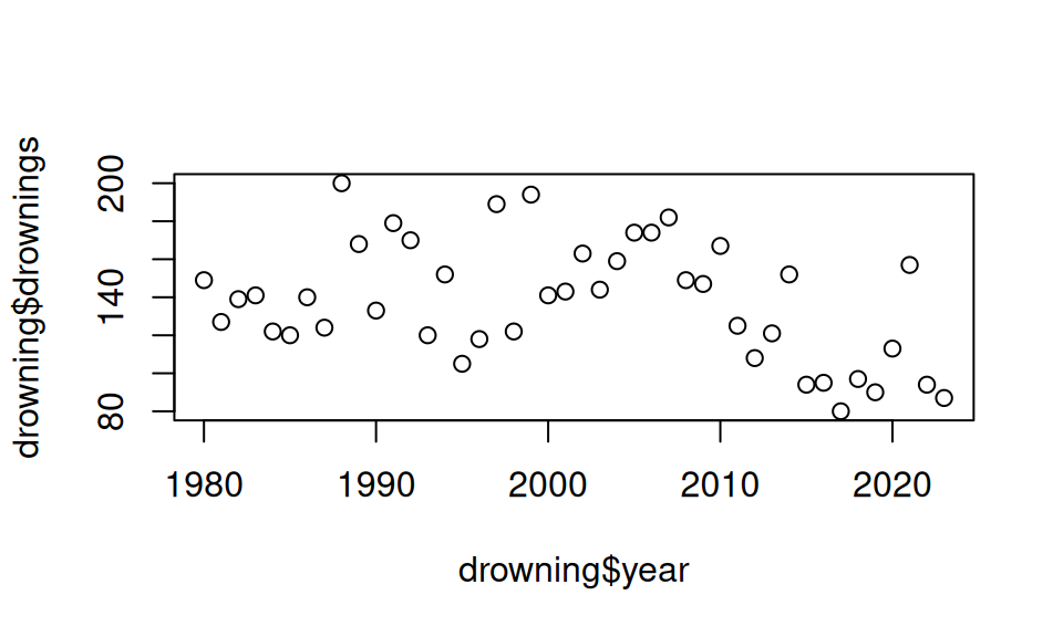
7 Plots
Include plots, with a specific width and height for the figure. We can also add label and caption for the plot:
Or using (more modern) ggplot() from ggplot2 package with pipe |>
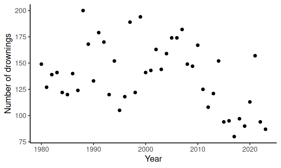
Or using ggplot() from ggplot2 package without pipe. In the following code bloc eval=FALSE is used to show the code, but not display the same plot again.
You can then refer the figure using @yourlabel-syntax: Figure 1, Figure 2. Figure labels should start with fig- prefix. If you label equations or tables, they should start witheq- and tbl- prefixes respectively.
8 Images
You can include an existing image (e.g. scanned copy of pen and paper equations). We will also add a label for cross-referencing.
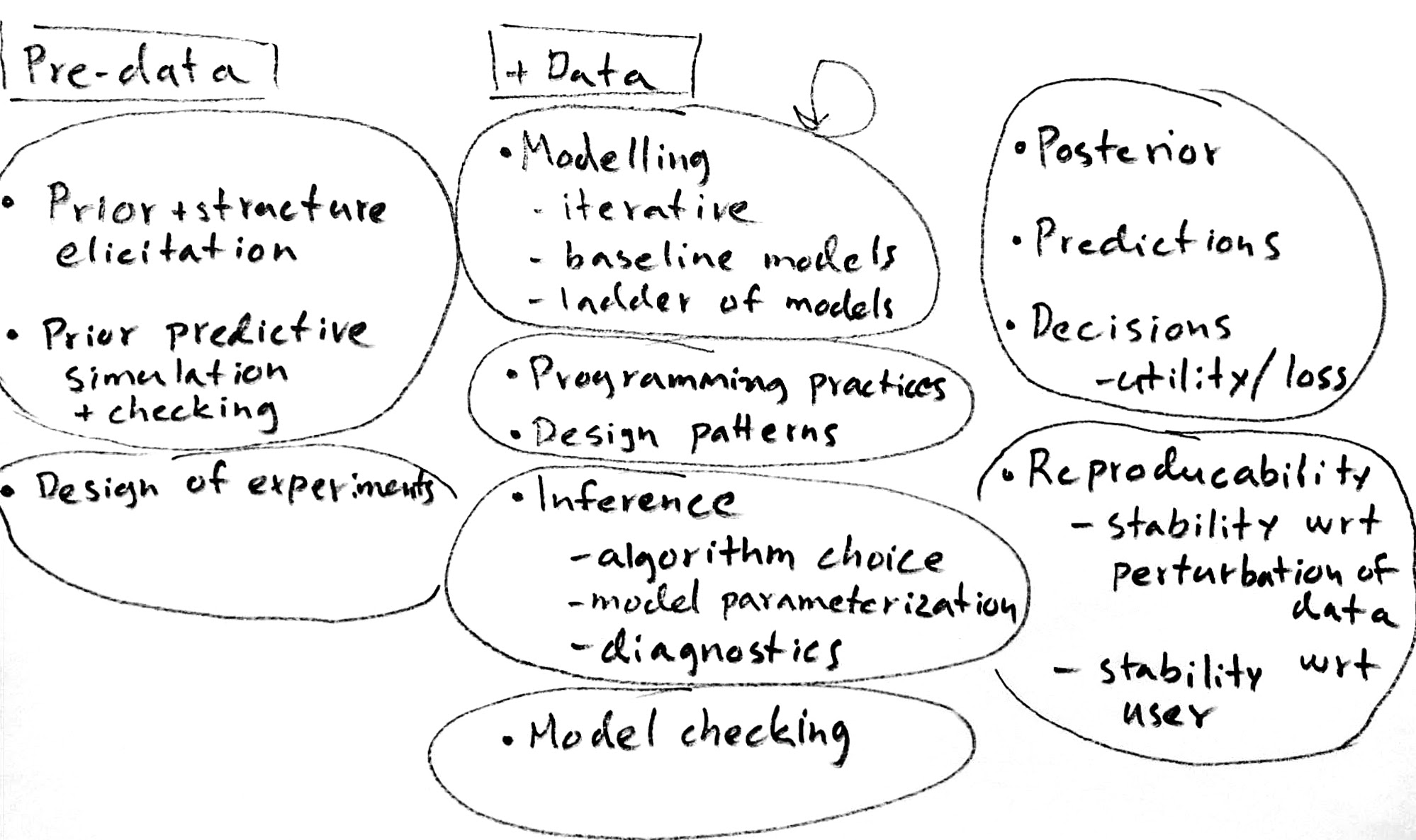
See Figure 3 for illustration of parts of Bayesian workflow.
9 Equations
You can write equations using LaTeX syntax, or you can include them as images if, for example, you use Microsoft Equations.
In Markdown, equations can easily be formulated using LaTeX in line as \(f(k) = {n \choose k} p^{k} (1-p)^{n-k}\). Or use the math environment as follows:
\[ \begin{array}{ccc} x_{11} & x_{12} & x_{13}\\ x_{21} & x_{22} & x_{23}. \end{array} \]
The above example illustrated also multicolumn ‘array’. Alternative way to make multiline equations with alignment is to use ‘aligned’ as follows:
\[ \begin{aligned} y & \sim \mathrm{normal}(\mu,1) \\ \mu & \sim \mathrm{normal}(0,1). \end{aligned} \]
Labeling equations allows to refer them later in the text. For example:
\[ p(\theta | y) = \frac{p(y | \theta )p(\theta)}{p(y)} \tag{1}\]
Posterior distribution of \(\theta\) is given by Equation 1 .
If you are new to LaTeX equations, you could use the latext4technics equation editor to create LaTeX equations to include in the report.
A short introduction to equations in LaTeX can be found at https://www.overleaf.com/learn/latex/Mathematical_expressions.
10 Tables
You can use knitr::kable to add formatted tables. Captioning and labeling works similarly as with plots.
| Year | Drownings |
|---|---|
| 1980 | 149 |
| 1981 | 127 |
| 1982 | 139 |
| 1983 | 141 |
| 1984 | 122 |
| 1985 | 120 |
Compare this to raw output:
  year drownings
1 1980       149
2 1981       127
3 1982       139
4 1983       141
5 1984       122
6 1985       120
It is also possible to control the number of digits, which is helpful to improve readability:
| mpg | cyl | disp | hp | drat | wt | qsec | vs | am | gear | carb | |
|---|---|---|---|---|---|---|---|---|---|---|---|
| Mazda RX4 | 21.0 | 6 | 160 | 110 | 3.9 | 2.6 | 16.5 | 0 | 1 | 4 | 4 |
| Mazda RX4 Wag | 21.0 | 6 | 160 | 110 | 3.9 | 2.9 | 17.0 | 0 | 1 | 4 | 4 |
| Datsun 710 | 22.8 | 4 | 108 | 93 | 3.9 | 2.3 | 18.6 | 1 | 1 | 4 | 1 |
| Hornet 4 Drive | 21.4 | 6 | 258 | 110 | 3.1 | 3.2 | 19.4 | 1 | 0 | 3 | 1 |
| Hornet Sportabout | 18.7 | 8 | 360 | 175 | 3.1 | 3.4 | 17.0 | 0 | 0 | 3 | 2 |
| Valiant | 18.1 | 6 | 225 | 105 | 2.8 | 3.5 | 20.2 | 1 | 0 | 3 | 1 |
Refer the table in the usual way: see Table 1.
11 Language
The language used in the course is English. Hence the report needs to be written in English.
12 Jupyter Notebook and other report formats
You are allowed to use any format to produce your report, such as Jupyter Notebook, as long as you follow the formatting instructions in this template. Using Quarto with Jupyter Lab is also possible. See getting started guide for Jupyter Lab.