Error: (converted from warning) Setting LC_CTYPE failed, using "C"
Execution halted
Error: Failed to install 'aaltobda' from GitHub:
(converted from warning) installation of package '/var/folders/g6/bdv4dr4s6qq4zyxw2nzy26kr0000gn/T//Rtmp3uYwuD/file121f355845a3/aaltobda_0.1.tar.gz' had non-zero exit statusBayesian Data Analysis course - FAQ
How to use R and RStudio remotely
Option 1: Using R and RStudio via JupyterHub
This the recommended option, as everything is pre-installed and tested.
Instead of installing RStudio on your computer, you can use it in your web browser:
- Information about Aalto JupyterHub
- Go to jupyter.cs.aalto.fi
- Choose
CS-E5710 - Bayesian Data Analysis (2025) - In the Launcher click
RStudio - In the RStudio Files pane (bottom right) you can create folders for your work and upload files from your computer to the server
- The notebooks folder is the only persistent folder (stays there if you sign out) so save everything to that folder!
- You may get an error when uploading a large zip file, but uploading smaller zip files work. If you can’t upload demo zip file contact the course staff via Zulip.
- You may access your data as a network drive by SMB mounting it on your own computer - see Accessing JupyterHub data. This allows you to have total control over your data.
- After uploading files, use Files pane to open them (e.g. an RMarkdown or Quarto notebook)
- Knitting of R, Rmd, and qmd files works as well (tested 24th August)
- CmdStanR used later in the course has been tested to work 24th August.
- To use CmdStanR:
library(cmdstanr)
- If you do not see the following output, please contact us on Zulip:
This is cmdstanr version 0.6.0
- CmdStanR documentation and vignettes: mc-stan.org/cmdstanr
- CmdStan path: /coursedata/cmdstan
- CmdStan version: 2.33.0
- If you do not see the following output, please contact us on Zulip:
- To use CmdStanR:
- There is a limited memory available (3Gib) and bigger models and datasets can run out of memory with cryptic error message, but the demos and assignment models should run (if not, then contact the course staff via Zulip).
- See also Aalto JupyterHub FAQ and bugs
Option 2: Use Aalto Linux via remote-desktop solution provided by Aalto-IT.
- Information about Aalto remote desktop
- Go to vdi.aalto.fi
- Download VMWare Horizon application or use the web portal
- If using the VMWare Horizon application, click on
New Serverand entervdi.aalto.fi
- If using the VMWare Horizon application, click on
- Enter your aalto username (aalto email works too) and password in the respective fields.
- Select
Ubuntu 20.04 - Click Activities, start typing
RStudioin the search bar, and clickRStudio.
How to access the BDA R (and Python) demos on CS JupyterHub
Go to
jupyter.cs.aalto.fion your favorite web-browser.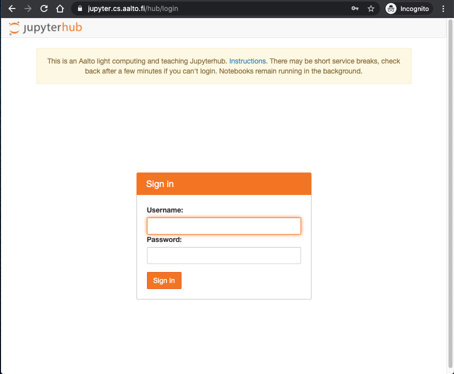
Log-in with your aalto username and password.
Select the
CS-E5710 - Bayesian Data Analysis (2025) -r-ubuntu:6.2.3-bayesda2025server.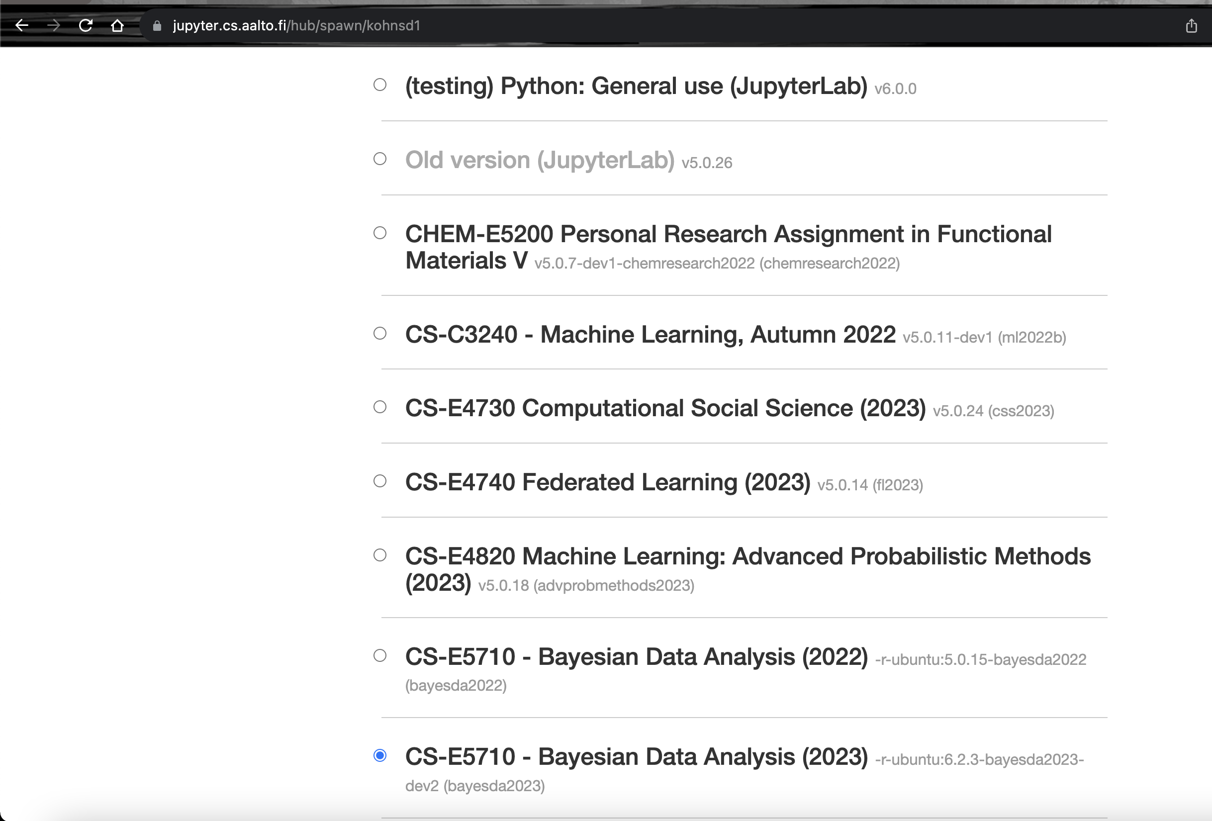
Select the
notebooksfolder in the left hand file browser.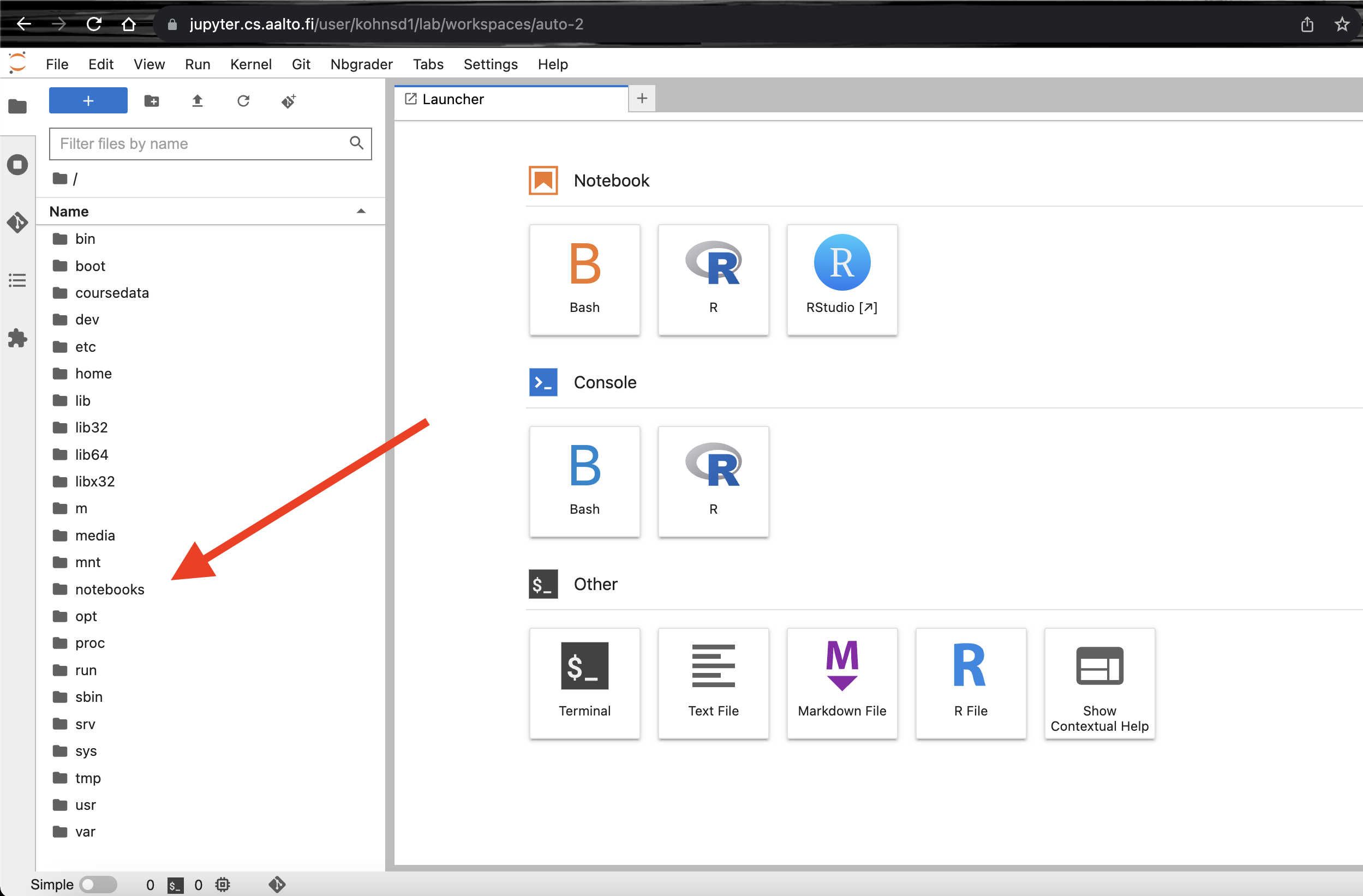
Select the
git clone iconas seen in the screenshot below.
In the text box type
https://github.com/avehtari/BDA_R_demos.gitfor python demos replaceBDA_R_demos.gitwithBDA_Python_demos.gitinstead. Then clickclone.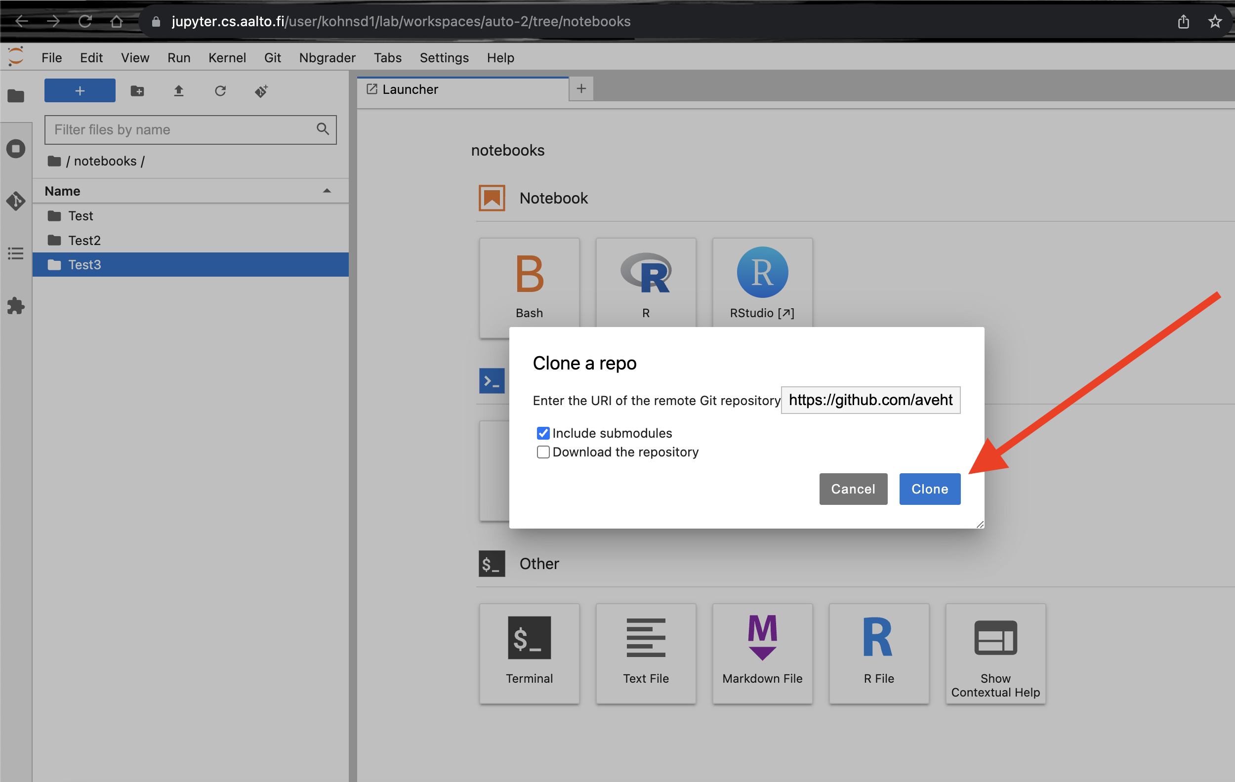
Wait a while, there should be
BDA_R_demosfolder undernotebooksfolder. Click on theBDA_R_demosfolder.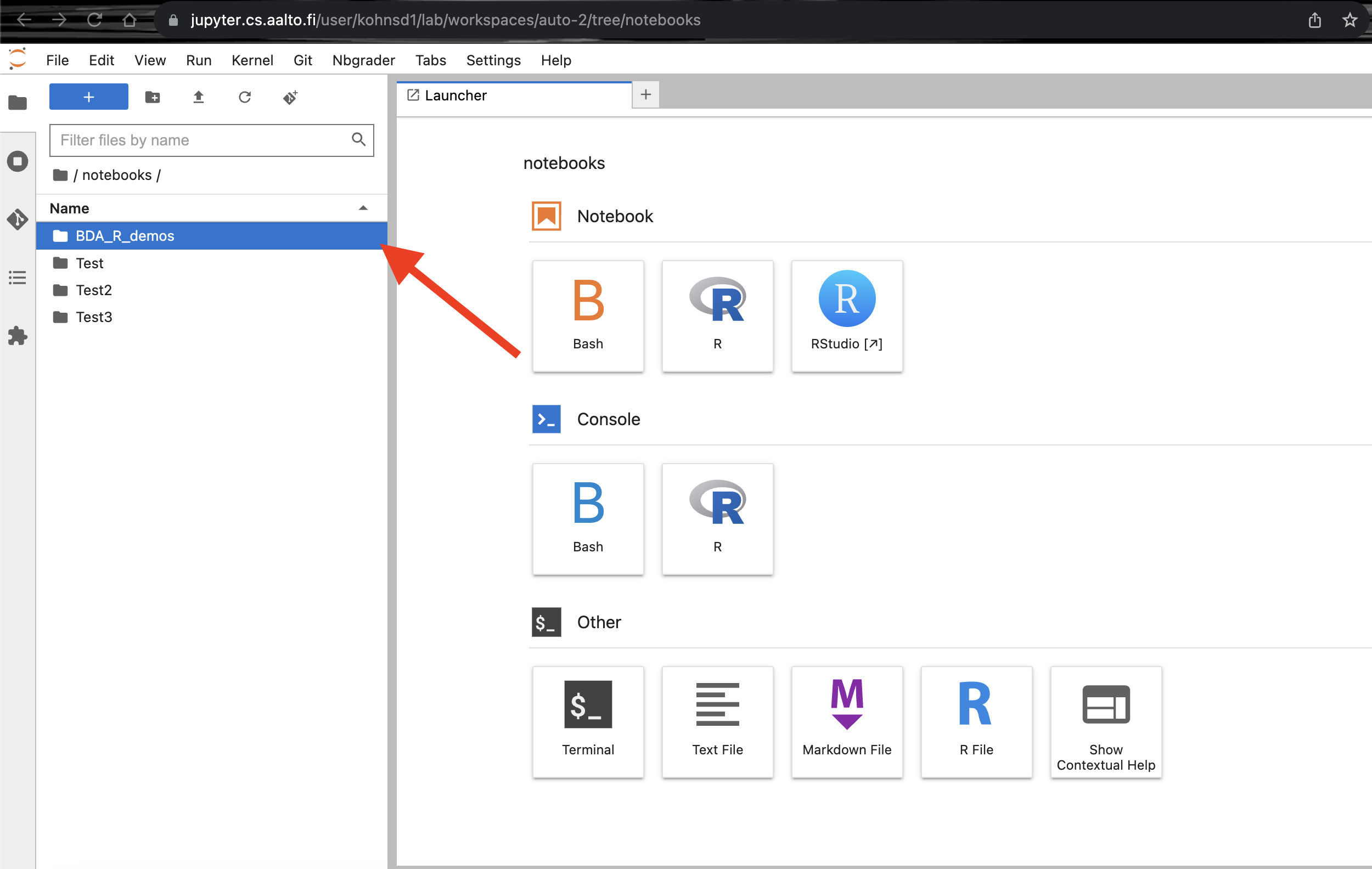
Click on the RStudio button on the right.
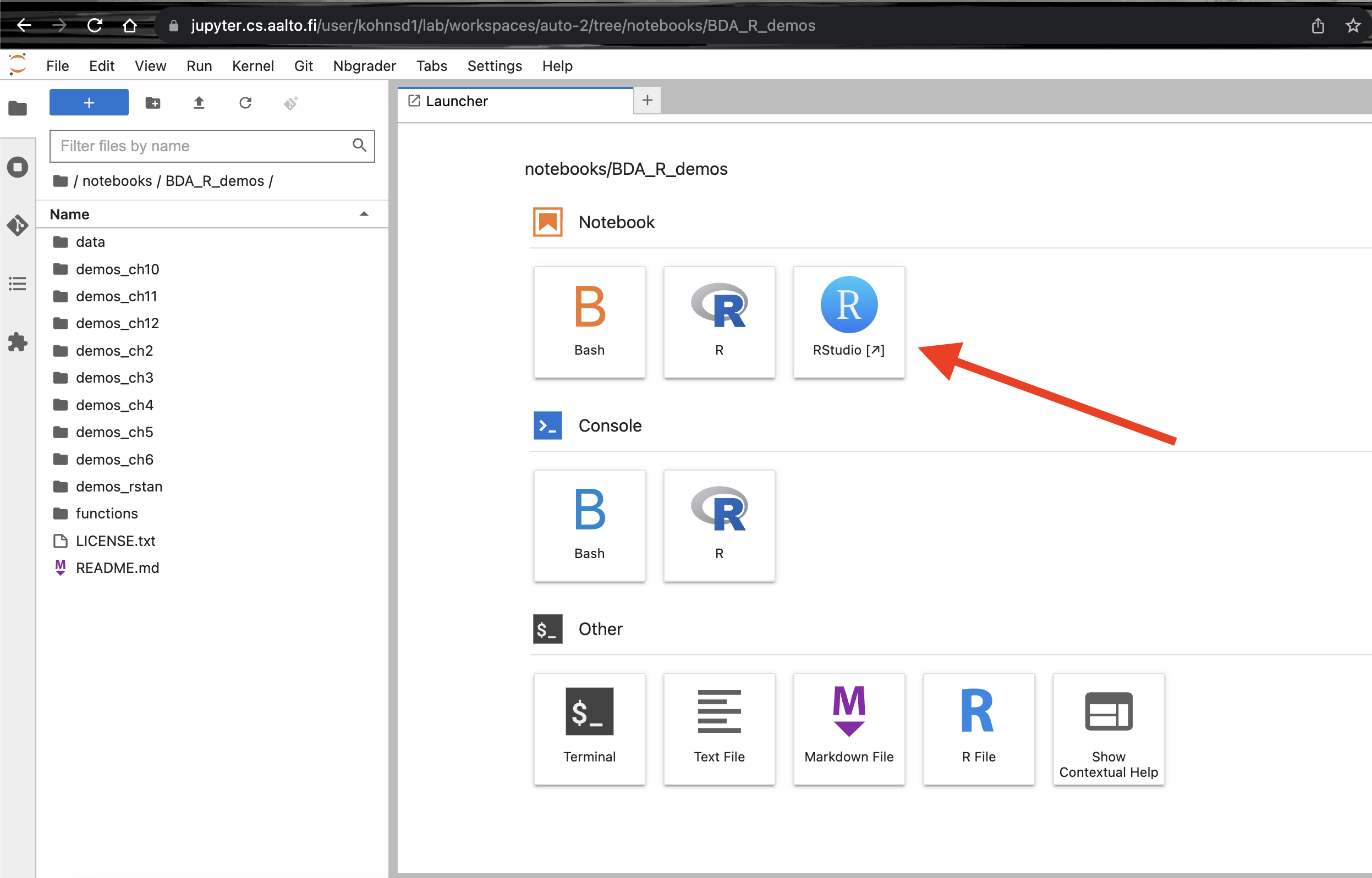
Now you should have an R-studio like interface in your web-browser. Click on
File -> Open File...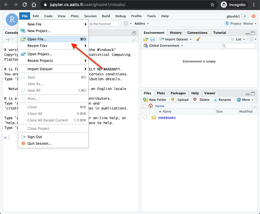
Click on
notebooksand then selectBDA_R_demosfolder.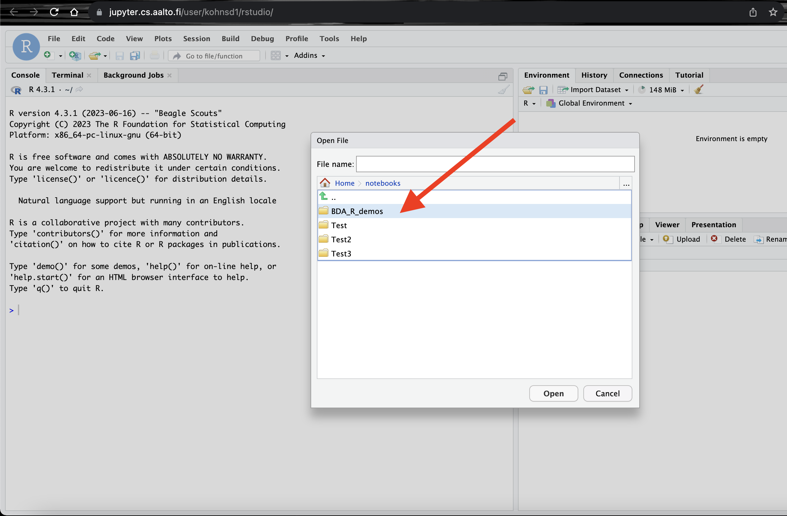
Select a demo to run. Here we open the folder
demos_ch2and then selectdemo2_1.Rfile and clickopen. This should open the file in the window.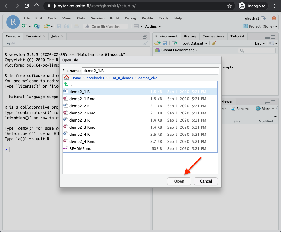
Select the contents of the file and click
Code -> Run Selected Line(s)as shown in the screenshot below.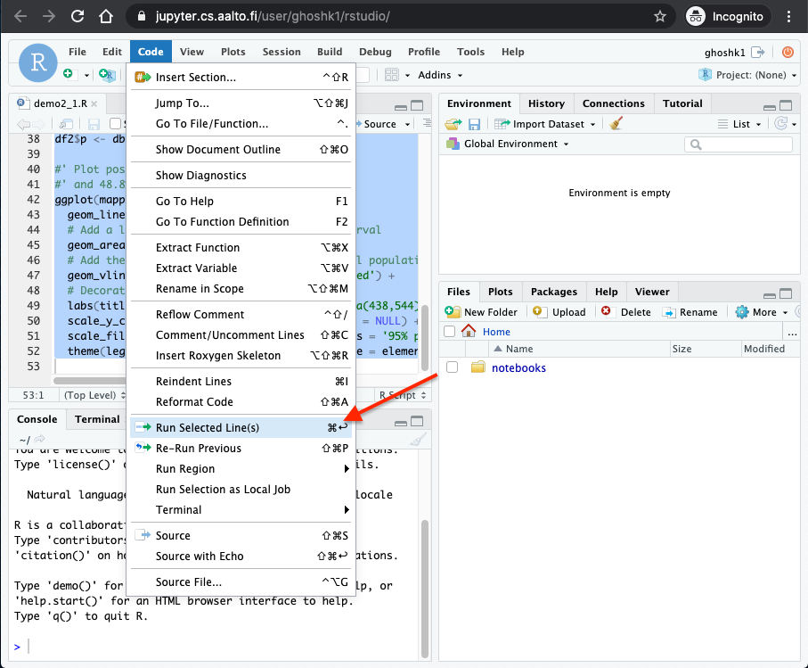
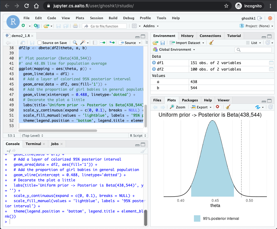
You should see the output of the code in the bottom right corner.
How to use R and RStudio on your own computer
How to access the course material in Github
Instead of trying to download each file separately via the Github interface, it is recommended to use one of these options:
- The best way is to clone the repository using git, and use pull to get the latest updates.
- If you want to learn to use git, start by installing a git client. There are plenty of good git tutorials online. See for example the tutorial by Aalto Git Aalto
- If you don’t want to learn to use git, download a the repository as a zip file. Click the green button “Code” at the main page of the repository and choose “Download ZIP” (direct link). Remember to download again during the course to get the latest updates.
R packages used in demos
Aalto JupyterHub has all the R packages used in demos pre-installed. If you install R on your own computer, you can install all the packages used by the main demos with
install.packages(c("MASS", "bayesplot", "brms", "cmdstanr ", "dplyr", "gganimate", "ggdist", "ggforce", "ggplot2", "grid", "gridExtra", "latex2exp", "loo", "plyr", "posterior", "purrr", "rprojroot", "tidyr", "quarto"))Installing aaltobda package
The course has its own R package aaltobda with data and functionality to simplify coding. aaltobda has been pre-installed in Aalto JupyterHub. To install the package to your own computer just run the following:
install.packages("aaltobda", repos = c("https://avehtari.r-universe.dev", getOption("repos")))
If during the course there is announcement that aaltobda has been updated (e.g. some error has been fixed), you can get the latest version by repeating the second step above.
Problems installing R packages on Windows ?
Getting the setup needed for the course working on Windows might involve a bit more effort than on Linux and Mac. Consequently, we recommend using either Linux or MacOS, or using R remotely. Moreover, Stan, the probabilistic programming language which we will use later on during the course requires a C++ compiler toolchain which is not available by default in Windows (blame Microsoft). However, if you want to use Windows and have a problem getting the setup working, below are two options to consider:
Installing knitr
If you just installed RStudio and R, chances are you don’t have knitr installed, the package responsible for rendering your notebook to pdf.
Solution:
install.packages("knitr")You can also install packages from RStudio menu Tools->Install Packages.
If knitr is installed but the pdf won’t compile
In this case it is possible that you don’t have LaTeX installed, which is the package that runs the engine to process the text and render the pdf itself.
Solution: Tinytex is the bare minimum Latex core that you need to install in order to run the pdf compiler. If you want to go further and download a full distribution of Latex, look at TeX Live for Linux and MacTeX for Mac OS.
install.packages("tinytex")
tinytex::install_tinytex()
How to install the latest version of CmdStanR or RStan
- Make sure you have installed R version 4.* or newer. If you don’t, install a newer version using instructions from https://www.r-project.org/
- At the moment
CmdStanRis faster in use, and thus we recommend usingCmdStanRinstead ofRStan, but both can be used for the assignments. CmdStanRis a lightweight interface to Stan for R users (seeCmdStanPyfor Python).CmdStanRavoids some installation problems as it doesn’t require matching C++ tools forRandRStan- Install
RStanalong with the necessary C++ compiler toolchain as described here
Instead of RStan, you can also use new CmdStanR which maybe easier to install.
Workarounds for current Rstan Windows issues
How to render a single qmd-file to html or pdf
Clicking Render in RStudio defaults to render all qmd files in the directory (“project”) and to render both html and pdf. To save time in rendering, you can install quarto R package
install.packages("quarto")
library(quarto)
and then render just one file and choose the target to be html with
quarto_render("template2.qmd", output_format = "html")and when you are ready to submit the pdf, use
quarto_render("template2.qmd", output_format = "pdf")quarto R package is available as pre-installed in JupyterHub (you may need to restart your server o get the new image).
If the rendering to pdf doesn’t work, you can print the html to pdf file, but do make sure to turn off “More setings -> Print headers and footers” to avoid accidentally printing your identity.
What is tidyr or tidyverse that is used in the R demos? What does %>% mean?
- Tidyverse is a collection of R packages designed for data science. The packages “share an underlying design philosophy, grammar, and data structures”.
- A clear characteristic that distinguishes tidyverse from the base R is the pipe operator
%>% - Recent R versions have a new built-in pipe operator
|>, which in most cases can replace%>%, and there are some differences only in more advanced use cases. - In this course you do not need to use tidyverse. However, some packages belonging to tidyverse, such as
ggplot2, can be useful for visualizing results in the reports.
M1 Macs with Python and Stan
Unfortunately the installation of pystan will fail on an M1 Mac, as there is not a binary wheel available for the httpstan dependency. A recommended alternative here is the CmdStanPy package.
M1 Mac users that are intent on using pystan will need to complete the following steps to build httpstan from source and then install pystan:
Build and Install httpstan
# Download httpstan source
git clone https://github.com/stan-dev/httpstan
cd httpstan
# Build shared libraries and generate code
python3 -m pip install poetry
# Build httpstan source
#   - There will be many compiler warnings, these are safe to ignore
make -j8
# Build the httpstan wheel
python3 -m poetry build
# Install the wheel
python3 -m pip install dist/*.whl
Install pystan
python3 -m pip install pystanI missed some deadline or wasn’t able to do some part of the course
- Can I combine results from assignments, project, presentation, and e-exam made in different periods / years?
- Yes.
- I missed the deadline to register for the course in Sisu. Can I join the course?
- Yes, just register in MyCourses and contact student services that they add you in Sisu, too.
- I missed the deadline for the assignment. Can you accept my late submission?
- Open MyCourses Quizzes are automatically submitted at the deadline time <!–
- If you miss the FeedbackFruits deadline first time it’s used due technical problems, but you send the pdf to one of the TAs few minutes after the deadline it can accepted once. As the recommended submission time is before 4pm on Friday, you have in general 56 hours extra hours for submission and several few minute late submissions is not likely just due to the technical problems. –>
- I was not able to do one of the assignments because [some personal problem]. Can I do some extra work?
- Things happen and you don’t need to tell the course staff your personal reasons (especially you shouldn’t tell any health issue details). Everyone gets a second change in period III. In period III there is just one submission deadline, but otherwise the procedure is the same. If you submitted the project work in autumn you don’t need to re-submit it if you re-submit assignments.
- I missed the deadline to register project group. Can I still register?
- Yes. Those who registered early are allowed to choose the presentation slots first.
- My group member a) disappeared, b) doesn’t do anything, c) is annoying. Can I continue with the project alone.
- First we hope you can resolve the issue, but if nothing works, then you can continue the project work alone.
- I was not able a) to do the project or b) to give a presentation because [some personal problem]. Can a) I submit it later, b) present later.
- Things happen and you don’t need to tell the course staff your personal reasons (especially you shouldn’t tell any health issue details). Everyone gets a second change in period III. In period III there is second project submission deadline and presentation slots. If you are happy with your assignment score, you don’t need to re-submit assignments if you submit the project work in period III.
Recommended courses after Bayesian Data Analysis
Here are some great Aalto courses that are using Bayesian inference
- CS-E4820 - Machine Learning: Advanced Probabilistic Methods (common probabilistic models in machine learning, such as sparse Bayesian linear models, Gaussian mixture models and factor analysis models, variational inference)
- ELEC-E8106 - Bayesian Filtering and Smoothing (dynamical systems, time series, tracking)
- CS-E4895 - Gaussian Processes
- CS-E5795 - Computational Methods in Stochastics (more about MC, MCMC, HMC)
- MS-E1654 - Computational Inverse Problems