---
title: "Notebook for Assignment 9"
author: "Aki Vehtari et al."
format:
html:
toc: true
code-tools: true
code-line-numbers: true
number-sections: true
mainfont: Georgia, serif
editor: source
---
# General information
This assignment relates to Lectures 9-10 and Chapter 9 of BDA3
We recommend using [JupyterHub](https://jupyter.cs.aalto.fi) (which has all the needed packages pre-installed).
::: hint
**Reading instructions:**
- [**For background on Bayes-R2**](https://acris.aalto.fi/ws/portalfiles/portal/34206843/bayes_R2_v3.pdf)
- [**The reading instructions for BDA3 Chapter 9**](../BDA3_notes.html#ch9) (decision analysis).
:::
{{< include includes/_general_cloze_instructions.md >}}
```{r}
if (!require(brms)) {
    install.packages("brms")
    library(brms)
}
if(!require(cmdstanr)){
    install.packages("cmdstanr", repos = c("https://mc-stan.org/r-packages/", getOption("repos")))
    library(cmdstanr)
}
cmdstan_installed <- function(){
  res <- try(out <- cmdstanr::cmdstan_path(), silent = TRUE)
  !inherits(res, "try-error")
}
if(!cmdstan_installed()){
    install_cmdstan()
}

if(!require(ggplot2)){
    install.packages("ggplot2")
    library(ggplot2)
}
if(!require(bayesplot)){
    install.packages("bayesplot")
    library(bayesplot)
}
if(!require(dplyr)){
    install.packages("dplyr")
    library(dplyr)
}
if(!require(tidyr)){
    install.packages("tidyr")
    library(tidyr)
}
if(!require(matrixStats)){
    install.packages("matrixStats")
    library(matrixStats)
}
if(!require(ggdist)){
    install.packages("ggdist")
    library(ggdist)
}
if(!require(tinytable)){
    install.packages("tinytable")
    library(tinytable)
}
if(!require(posterior)){
    install.packages("posterior")
    library(posterior)
}
if(!require(patchwork)){
    install.packages("patchwork")
    library(patchwork)
}
if(!require(mvtnorm)){
    install.packages("mvtnorm")
    library(mvtnorm)
}
theme_set(bayesplot::theme_default(base_family = "sans"))
```
# R2
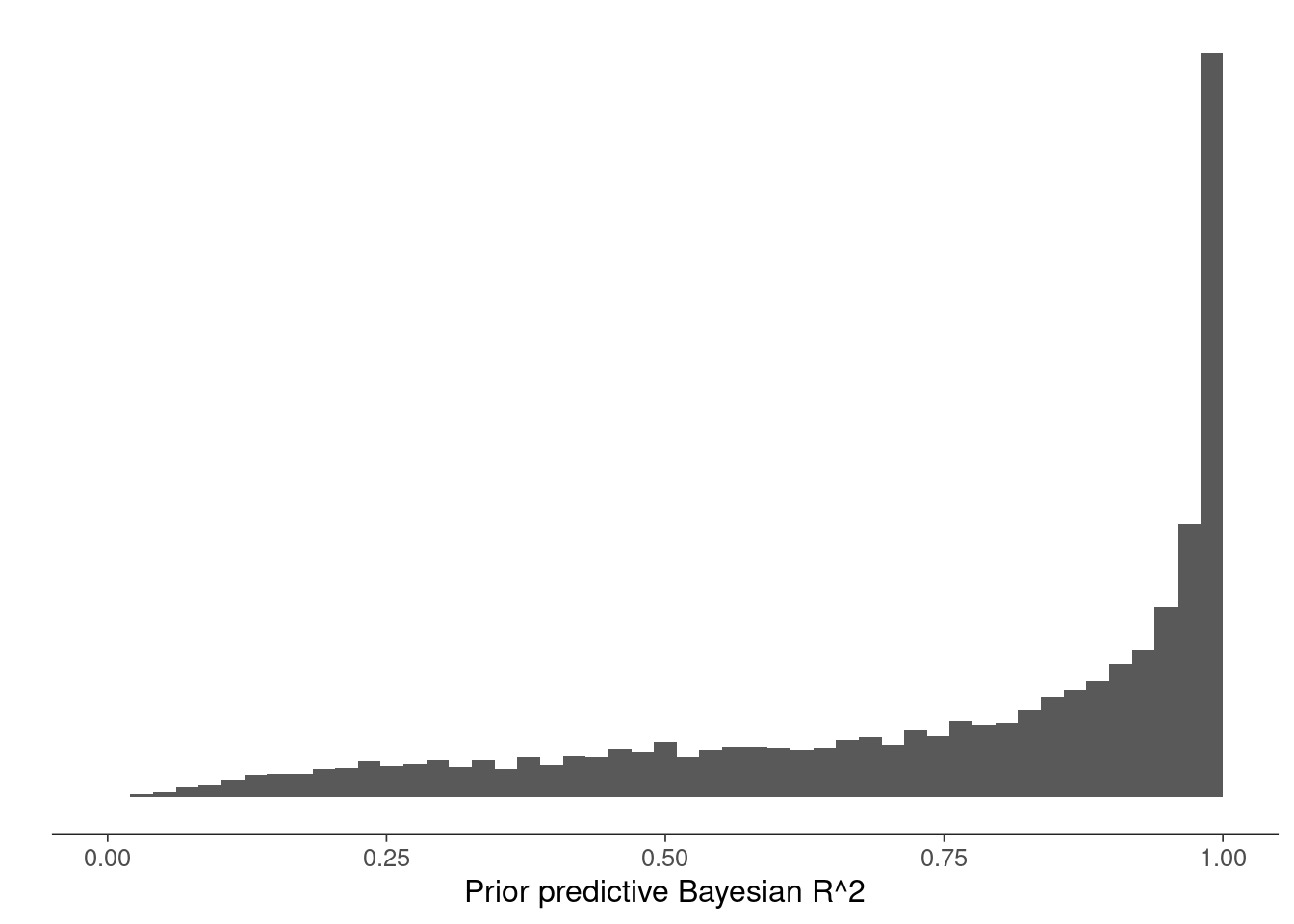
Compute and plot the prior predictive R2 distributions for the standard normal prior and R2 prior normal models. Modify the code below.
```{r}
sims <- 10000
p <- 26
n <- 400
X <- rmvnorm(n,mean = array(0,p),sigma = diag(array(1,p)))


## Prior Predictive Graphs: Normal
ppR2_gausprior<-numeric()

for (i in 1:sims) {
  sigma2 <- rexp(1,rate=1/3)^2
  beta <- rnorm(p)
  mu <- X%*%as.vector(beta)
  muvar <- var(mu)
  ppR2_gausprior[i] <- muvar/(muvar+sigma2)
}
ggplot()+geom_histogram(aes(x=ppR2_gausprior), breaks=seq(0,1,length.out=50)) +
  xlim(c(0,1)) +
  scale_y_continuous(breaks=NULL) +
  labs(x="Prior predictive Bayesian R^2",y="")
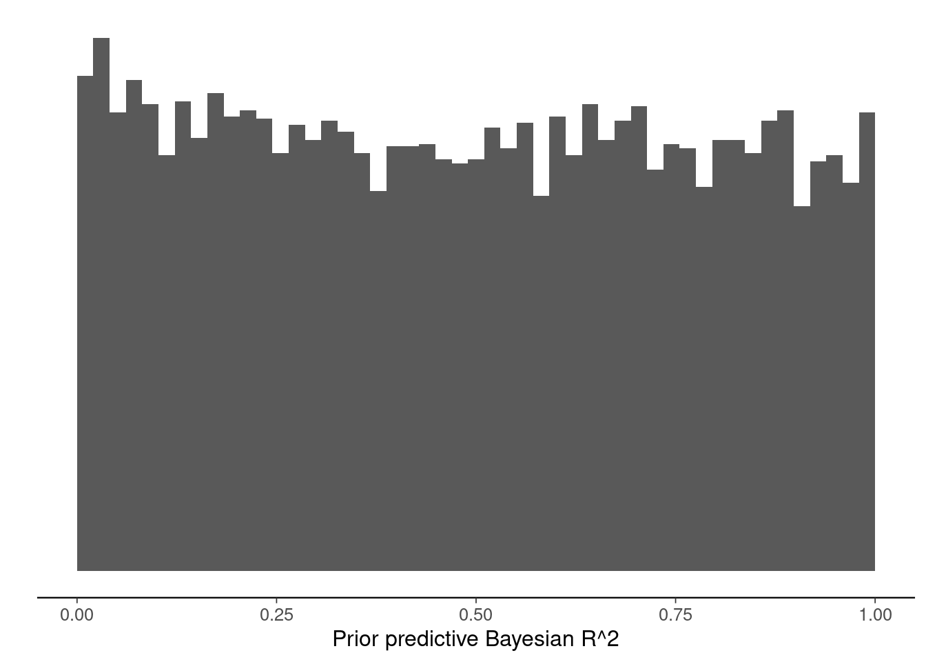
## Prior Predictive Graphs: R^2 prior
ppR2_r2prior<-numeric()
mu_R2 <- 0.5
scale_R2 <- 2

for (i in 1:sims) {
  sigma2 <- rexp(1,rate=1/3)^2
  R2 <- rbeta(1,(mu_R2*scale_R2),((1-mu_R2)*scale_R2))
  tau2 <- R2/(1-R2)
  psi <- rdirichlet(1,rep(1,p))
  beta <- rnorm(p) * sqrt(tau2*psi*sigma2)
  mu <- X%*%as.vector(beta)
  muvar <- var(mu)
  ppR2_r2prior[i] <- muvar/(muvar+sigma2)
}
ggplot()+geom_histogram(aes(x=ppR2_r2prior), breaks=seq(0,1,length.out=50)) +
  xlim(c(0,1)) +
  scale_y_continuous(breaks=NULL) +
  labs(x="Prior predictive Bayesian R^2",y="")
```
# Portuguese Student Data
## Data Prep
```{r}
# Load the data
student <- read.csv(url('https://raw.githubusercontent.com/avehtari/ROS-Examples/master/Student/data/student-merged.csv'))

# Predictors to be used
predictors <- c("school","sex","age","address","famsize","Pstatus","Medu","Fedu","traveltime","studytime","failures","schoolsup","famsup","paid","activities", "nursery", "higher", "internet", "romantic","famrel","freetime","goout","Dalc","Walc","health","absences")
p <- length(predictors)

# To reduce variability us the median grades based on those three
# exams for each topic, students with non-zero grades are selected
grades <- c("G1mat","G2mat","G3mat","G1por","G2por","G3por")
student <- student %>%
  mutate(across(matches("G[1-3]..."), ~na_if(.,0))) %>%
  mutate(Gmat = rowMedians(as.matrix(select(.,matches("G.mat"))), na.rm=TRUE),
         Gpor = rowMedians(as.matrix(select(.,matches("G.por"))), na.rm=TRUE))
student_Gmat <- subset(student, is.finite(Gmat), select=c("Gmat",predictors))
student_Gmat <- student_Gmat[is.finite(rowMeans(student_Gmat)),]
student_Gpor <- subset(student, is.finite(Gpor), select=c("Gpor",predictors))
(nmat <- nrow(student_Gmat))
# Look at the data
head(student_Gmat) |> tt()
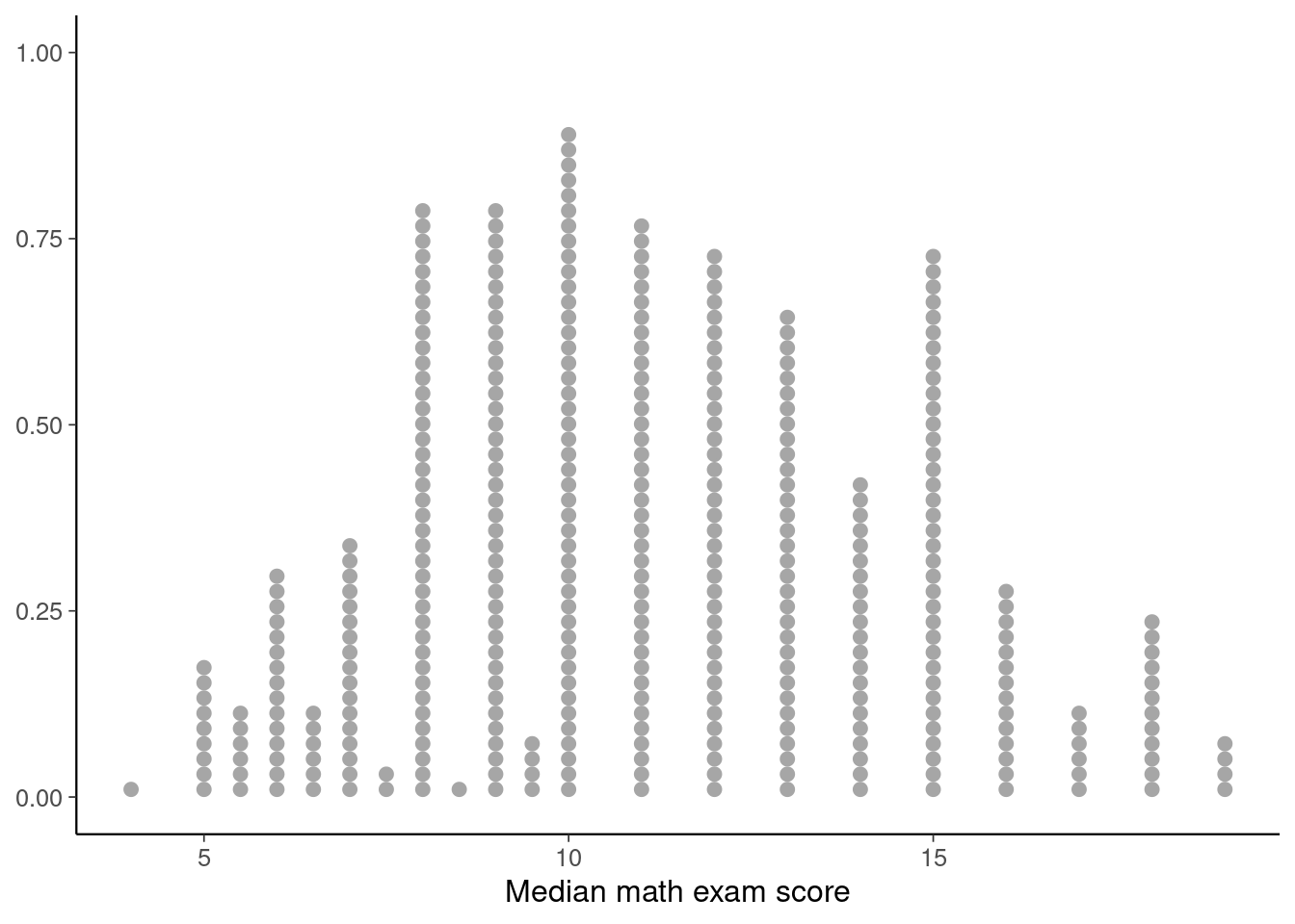
# Visualise the distributions of median math scores
p1 <- ggplot(student_Gmat, aes(x=Gmat)) + geom_dots() + labs(x='Median math exam score')
p1
# Some data transformation for non-binary predictors to have standard
# deviation 1
studentstd_Gmat <- student_Gmat
Gmatbin<-apply(student_Gmat[,predictors], 2, function(x) {length(unique(x))==2})
studentstd_Gmat[,predictors[!Gmatbin]] <-scale(student_Gmat[,predictors[!Gmatbin]])
studentstd_Gpor <- student_Gpor
Gporbin<-apply(student_Gpor[,predictors], 2, function(x) {length(unique(x))==2})
studentstd_Gpor[,predictors[!Gporbin]] <-scale(student_Gpor[,predictors[!Gporbin]])

# Set Seed for reproducibility
SEED <- 2132
```
## Normal Model
Estimate model
```{r}
# Estimate Model
fit1 <- brm(Gmat ~ ., data = studentstd_Gmat,
             normalize=FALSE,
            seed = SEED)
```
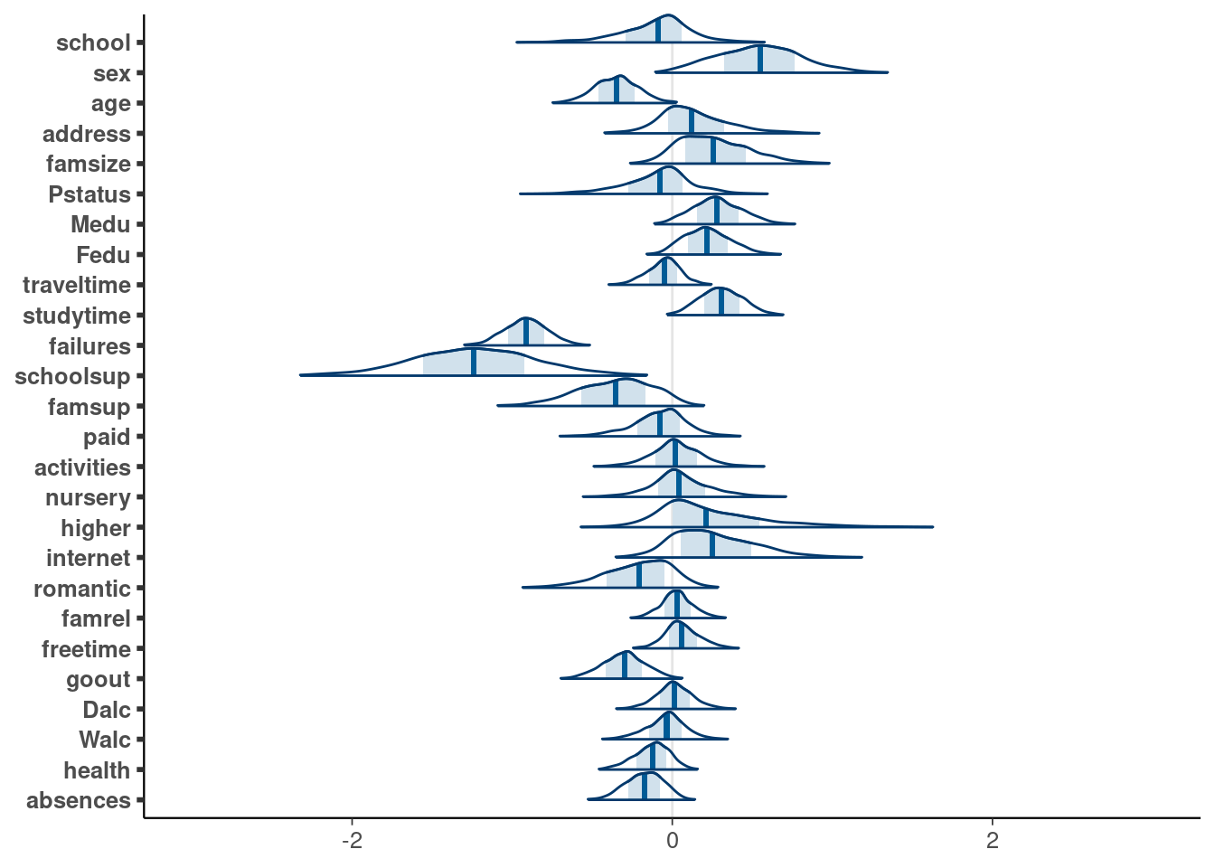
Visualise posteriors
```{r}
# Plot marginal posteriors of the coefficients
drawsmu <- as_draws_df(fit1, variable=paste0('b_',predictors)) |>
  set_variables(predictors)
p <- mcmc_areas(drawsmu,
                prob_outer=0.98, area_method = "scaled height") +
  xlim(c(-3,3))
p <- p + scale_y_discrete(limits = rev(levels(p$data$parameter)))
p
```
Now, find prior predictive R2
```{r}
X <- studentstd_Gmat[,2:dim(student_Gmat)[2]]

ppR2_1<-numeric()
sims <- 4000

for (i in 1:sims) {
  sigma2 <- rstudent_t(1,3,0,3)^2
  beta <- rnorm(length(predictors))
  mu <- as.matrix(X)%*%as.vector(beta)
  muvar <- var(mu)
  ppR2_1[i] <- muvar/(muvar+sigma2)
}
```
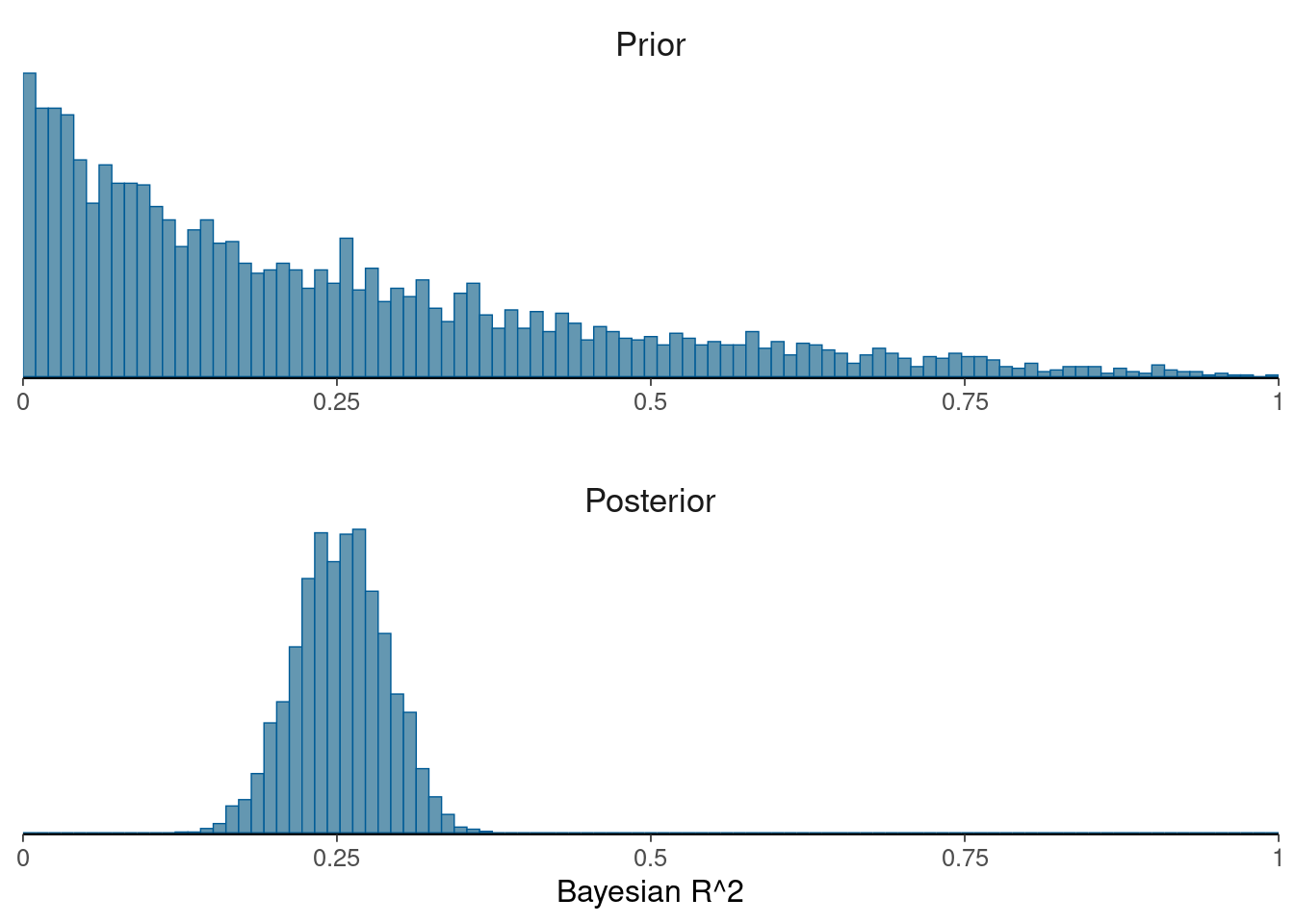
Plot prior predictive R2 vs posterior R2
```{r}
data <- data.frame(Prior=ppR2_1,Posterior=bayes_R2(fit1, summary=FALSE))
names(data) <- c("Prior","Posterior")
mcmc_hist(data,
          breaks=seq(0,1,length.out=100),
          facet_args = list(nrow = 2)) +
  facet_text(size = 13) +
  scale_x_continuous(limits = c(0,1), expand = c(0, 0),
                     labels = c("0","0.25","0.5","0.75","1")) +
  theme(axis.line.y = element_blank()) +
  xlab("Bayesian R^2")
```
Bayes-R2 and LOO-R2
```{r}
bayes_R2(fit1) |> as.data.frame() |> tt()
loo_R2(fit1) |> as.data.frame() |> tt()
```
## R2 Model
Estimate the model, amend the code below
```{r}
fit2 <- brm(Gmat ~ ., data = studentstd_Gmat,
            seed = SEED,
            normalize = FALSE,
            prior=c(prior(R2D2(mean_R2 = 0.5, prec_R2 = 1, cons_D2 = 1,
                               autoscale = TRUE),class=b)),
            backend = "cmdstanr")
```
Visualise Posteriors
```{r}
# Plot marginal posteriors
draws2 <- as_draws_df(fit2, variable=paste0('b_',predictors)) |>
  set_variables(predictors)
p <- mcmc_areas(draws2,
                prob_outer=0.98, area_method = "scaled height") +
  xlim(c(-3,3))
p <- p + scale_y_discrete(limits = rev(levels(p$data$parameter)))
p
```
Find prior predictive R2. This should be equal to the prior you set on R2 if all predictors are scaled to have unit variance. Since binary predictors were not standardised, the prior predictive might look slightly different, let's compute it for illustration
```{r}
ppR2_2<-numeric()
sims <- 4000

for (i in 1:sims) {
  sigma2 <- rstudent_t(1,3,0,3)^2
  R2 <- rbeta(1,1,2)
  tau2 <- R2/(1-R2)
  psi <- as.numeric(rdirichlet(1,rep(1,dim(X)[2])))
  beta <- rnorm(dim(X)[2])*sqrt(sigma2*tau2*psi)
  mu <- as.matrix(X)%*%as.vector(beta)
  muvar <- var(mu)
  ppR2_2[i] <- muvar/(muvar+sigma2)
}
```
Now, find the predictive R2 and compare to the posterior.
```{r}
# Prior vs posterior R2
data <- data.frame(Prior=ppR2_2,Posterior=bayes_R2(fit2, summary=FALSE))
names(data) <- c("Prior","Posterior")
mcmc_hist(data,
          breaks=seq(0,1,length.out=100),
          facet_args = list(nrow = 2)) +
  facet_text(size = 13) +
  scale_x_continuous(limits = c(0,1), expand = c(0, 0),
                     labels = c("0","0.25","0.5","0.75","1")) +
  theme(axis.line.y = element_blank()) +
  xlab("Bayesian R^2")
```
Summaries of R2 and LOO-R2
```{r}
# Bayes-R2 and LOO-R2
bayes_R2(fit2) |> as.data.frame() |> tt()
loo_R2(fit2) |> as.data.frame() |> tt()
```