1 Introduction

This notebook demonstrates Bayesian posterior distributions of model based R-squared and LOO-R2 measures for linear and logistic regression. This notebook is a supplement for the paper

Andrew Gelman, Ben Goodrich, Jonah Gabry, and Aki Vehtari (2018). R-squared for Bayesian regression models. The American Statistician, doi:10.1080/00031305.2018.1549100. Online Preprint.

We specifically define R-squared as \[ R^2 = \frac{{\mathrm Var}_{\mu}}{{\mathrm Var}_{\mu}+{\mathrm Var}_{\mathrm res}}, \] where \({\mathrm Var}_{\mu}\) is variance of modelled predictive means, and \({\mathrm Var}_{\mathrm res}\) is the modelled residual variance. Specifically both of these are computed only using posterior quantities from the fitted model.

The residual based R2 uses draws from the residual distribution and is defined as \[ {\mathrm Var}_{\mu}^s = V_{n=1}^N \hat{y}_n^s\\ {\mathrm Var}_{\mathrm res}^s = V_{n=1}^N \hat{e}_n^s, \] where \(\hat{e}_n^s=y_n-\hat{y}_n^s\).

The model based R2 uses draws from the modeled residual variances. For linear regression we define \[ {\mathrm Var}_{\mathrm res}^s = (\sigma^2)^s, \] and for logistic regression, following Tjur (2009), we define \[ {\mathrm Var}_{\mathrm res}^s = \frac{1}{N}\sum_{n=1}^N (\pi_n^s(1-\pi_n^s)), \] where \(\pi_n^s\) are predicted probabilities.

The LOO-R2 uses LOO residuals and is defined \(1-{\mathrm Var}_{\mathrm loo-res}/{\mathrm Var}_{y}\) and \[ {\mathrm Var}_{y} = V_{n=1}^N {y}_n\\ {\mathrm Var}_{\mathrm loo-res} = V_{n=1}^N \hat{e}_{{\mathrm loo},n}, \] where \(\hat{e}_{{\mathrm loo},n}=y_n-\hat{y}_{{\mathrm loo},n}\). The uncertainty in LOO-R2 comes from not knowing the future data distribution (Vehtari and Ojanen, 2012). We can approximate draws from the corresponding distribution using Bayesian bootstrap (Vehtari and Lampinen, 2002).

File contents:

bayes_R2_res function (using residuals)
bayes_R2 function (using sigma and latent space for binary)
loo_R2 function (using LOO residuals and Bayesian bootstrap for uncertainty)
code for fitting the models for the example in the paper
code for producing the plots in the paper (both base graphics and ggplot2 code)
several examples

Corresponding Bayes_R2.R file

Load packages

Data comes from the Regression and Other Stories examples which are included in the rosdata R package, which can be installed with remotes::install_github("avehtari/ROS-Examples",subdir = "rpackage")

library("rosdata")
library("rstanarm")
options(mc.cores = parallel::detectCores())
library("loo")
library("ggplot2")
library("bayesplot")
theme_set(bayesplot::theme_default(base_family = "sans"))
library("latex2exp")
library("foreign")
library("bayesboot")
SEED <- 1800
set.seed(SEED)

2 Functions for Bayesian R-squared for stan_glm models.

A more complicated version of this function that is compatible with stan_glmer models and specifying newdata will be available in the rstanarm package.

@param fit A fitted model object returned by stan_glm.
@return A vector of R-squared values with length equal to the number of posterior draws.

Bayes-R2 function using residuals

bayes_R2_res <- function(fit) {
  y <- rstanarm::get_y(fit)
  ypred <- rstanarm::posterior_epred(fit)
  if (family(fit)$family == "binomial" && NCOL(y) == 2) {
    trials <- rowSums(y)
    y <- y[, 1]
    ypred <- ypred %*% diag(trials)
  }
  e <- -1 * sweep(ypred, 2, y)
  var_ypred <- apply(ypred, 1, var)
  var_e <- apply(e, 1, var)
  var_ypred / (var_ypred + var_e)
}

Bayes-R2 function using modelled (approximate) residual variance

bayes_R2 <- function(fit) {
  mupred <- rstanarm::posterior_epred(fit)
  var_mupred <- apply(mupred, 1, var)
  if (family(fit)$family == "binomial" && NCOL(y) == 1) {
      sigma2 <- apply(mupred*(1-mupred), 1, mean)
  } else {
      sigma2 <- as.matrix(fit, pars = c("sigma"))^2
  }
  var_mupred / (var_mupred + sigma2)
}

LOO-R2 function using LOO-residuals and Bayesian bootstrap

loo_R2 <- function(fit) {
    y <- get_y(fit)
    ypred <- posterior_epred(fit)
    ll <- log_lik(fit)
    M <- length(fit$stanfit@sim$n_save)
    N <- fit$stanfit@sim$n_save[[1]]
    r_eff <- relative_eff(exp(ll), chain_id = rep(1:M, each = N))
    psis_object <- psis(log_ratios = -ll, r_eff = r_eff)
    ypredloo <- E_loo(ypred, psis_object, log_ratios = -ll)$value
    eloo <- ypredloo-y
    n <- length(y)
    rd<-rudirichlet(4000, n)
    vary <- (rowSums(sweep(rd, 2, y^2, FUN = "*")) -
             rowSums(sweep(rd, 2, y, FUN = "*"))^2)*(n/(n-1))
    vareloo <- (rowSums(sweep(rd, 2, eloo^2, FUN = "*")) -
                rowSums(sweep(rd, 2, eloo, FUN = "*")^2))*(n/(n-1))
    looR2 <- 1-vareloo/vary
    looR2[looR2 < -1] <- -1
    looR2[looR2 > 1] <- 1
    return(looR2)
}

3 Experiments

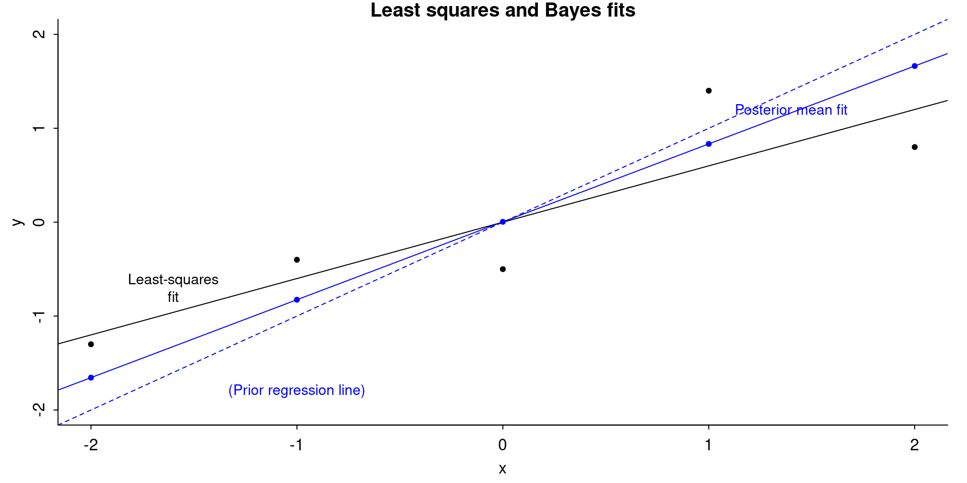
3.1 Toy data with n=5

x <- 1:5 - 3
y <- c(1.7, 2.6, 2.5, 4.4, 3.8) - 3
xy <- data.frame(x,y)

Lsq fit

fit <- lm(y ~ x, data = xy)
ols_coef <- coef(fit)
yhat <- ols_coef[1] + ols_coef[2] * x
r <- y - yhat
rsq_1 <- var(yhat)/(var(y))
rsq_2 <- var(yhat)/(var(yhat) + var(r))
round(c(rsq_1, rsq_2), 3)

[1] 0.766 0.766

Bayes fit

fit_bayes <- stan_glm(y ~ x, data = xy,
  prior_intercept = normal(0, 0.2, autoscale = FALSE),
  prior = normal(1, 0.2, autoscale = FALSE),
  prior_aux = NULL,
  seed = SEED,
  refresh = 0
)
posterior <- as.matrix(fit_bayes, pars = c("(Intercept)", "x"))
post_means <- colMeans(posterior)

Median Bayesian R2

round(median(bayesR2res<-bayes_R2_res(fit_bayes)), 2)

[1] 0.8

round(median(bayesR2<-bayes_R2(fit_bayes)), 2)

[1] 0.74

LOO-R2

looR2<-loo_R2(fit_bayes)

Warning: Some Pareto k diagnostic values are too high. See help('pareto-k-diagnostic') for details.

round(median(looR2), 2)

[1] 0.56

With small n LOO-R2 is much lower than median of Bayesian R2

Figures

The first section of code below creates plots using base R graphics.
Below that there is code to produce the plots using ggplot2.

# take a sample of 20 posterior draws
keep <- sample(nrow(posterior), 20)
samp_20_draws <- posterior[keep, ]

Base graphics version

par(mar=c(3,3,1,1), mgp=c(1.7,.5,0), tck=-.01)
plot(
  x, y,
  ylim = range(x),
  xlab = "x",
  ylab = "y",
  main = "Least squares and Bayes fits",
  bty = "l",
  pch = 20
)
abline(coef(fit)[1], coef(fit)[2], col = "black")
text(-1.6,-.7, "Least-squares\nfit", cex = .9)
abline(0, 1, col = "blue", lty = 2)
text(-1, -1.8, "(Prior regression line)", col = "blue", cex = .9)
abline(coef(fit_bayes)[1], coef(fit_bayes)[2], col = "blue")
text(1.4, 1.2, "Posterior mean fit", col = "blue", cex = .9)
points(
  x,
  coef(fit_bayes)[1] + coef(fit_bayes)[2] * x,
  pch = 20,
  col = "blue"
)

par(mar=c(3,3,1,1), mgp=c(1.7,.5,0), tck=-.01)
plot(
  x, y,
  ylim = range(x),
  xlab = "x",
  ylab = "y",
  bty = "l",
  pch = 20,
  main = "Bayes posterior simulations"
)
for (s in 1:nrow(samp_20_draws)) {
  abline(samp_20_draws[s, 1], samp_20_draws[s, 2], col = "#9497eb")
}
abline(
  coef(fit_bayes)[1],
  coef(fit_bayes)[2],
  col = "#1c35c4",
  lwd = 2
)
points(x, y, pch = 20, col = "black")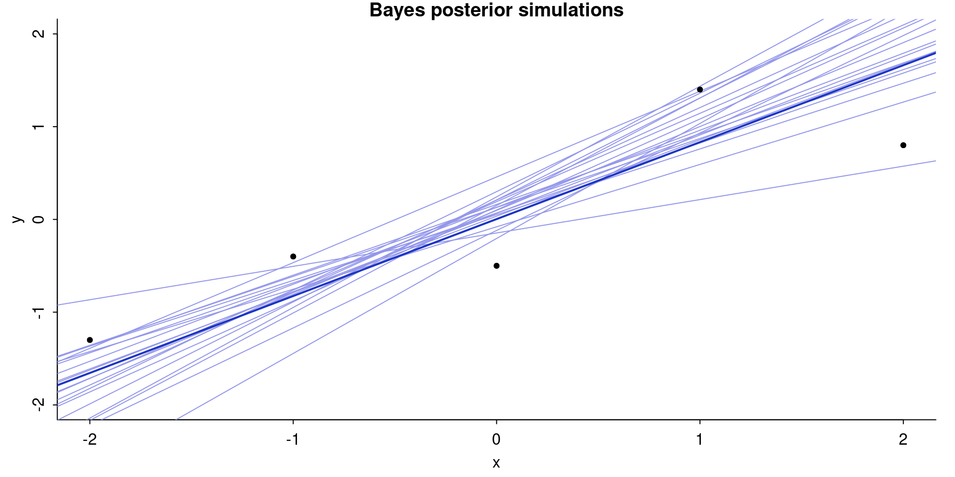

ggplot version

theme_update(
  plot.title = element_text(face = "bold", hjust = 0.5), 
  axis.text = element_text(size = rel(1.1))
)
fig_1a <-
  ggplot(xy, aes(x, y)) +
  geom_point() +
  geom_abline( # ols regression line
    intercept = ols_coef[1],
    slope = ols_coef[2],
    size = 0.4
  ) +
  geom_abline( # prior regression line
    intercept = 0,
    slope = 1,
    color = "blue",
    linetype = 2,
    size = 0.3
  ) +
  geom_abline( # posterior mean regression line
    intercept = post_means[1],
    slope = post_means[2],
    color = "blue",
    size = 0.4
  ) +
  geom_point(
    aes(y = post_means[1] + post_means[2] * x),
    color = "blue"
  ) +
  annotate(
    geom = "text",
    x = c(-1.6, -1, 1.4),
    y = c(-0.7, -1.8, 1.2),
    label = c(
      "Least-squares\nfit",
      "(Prior regression line)",
      "Posterior mean fit"
    ),
    color = c("black", "blue", "blue"),
    size = 3.8
  ) +
  ylim(range(x)) + 
  ggtitle("Least squares and Bayes fits")
plot(fig_1a)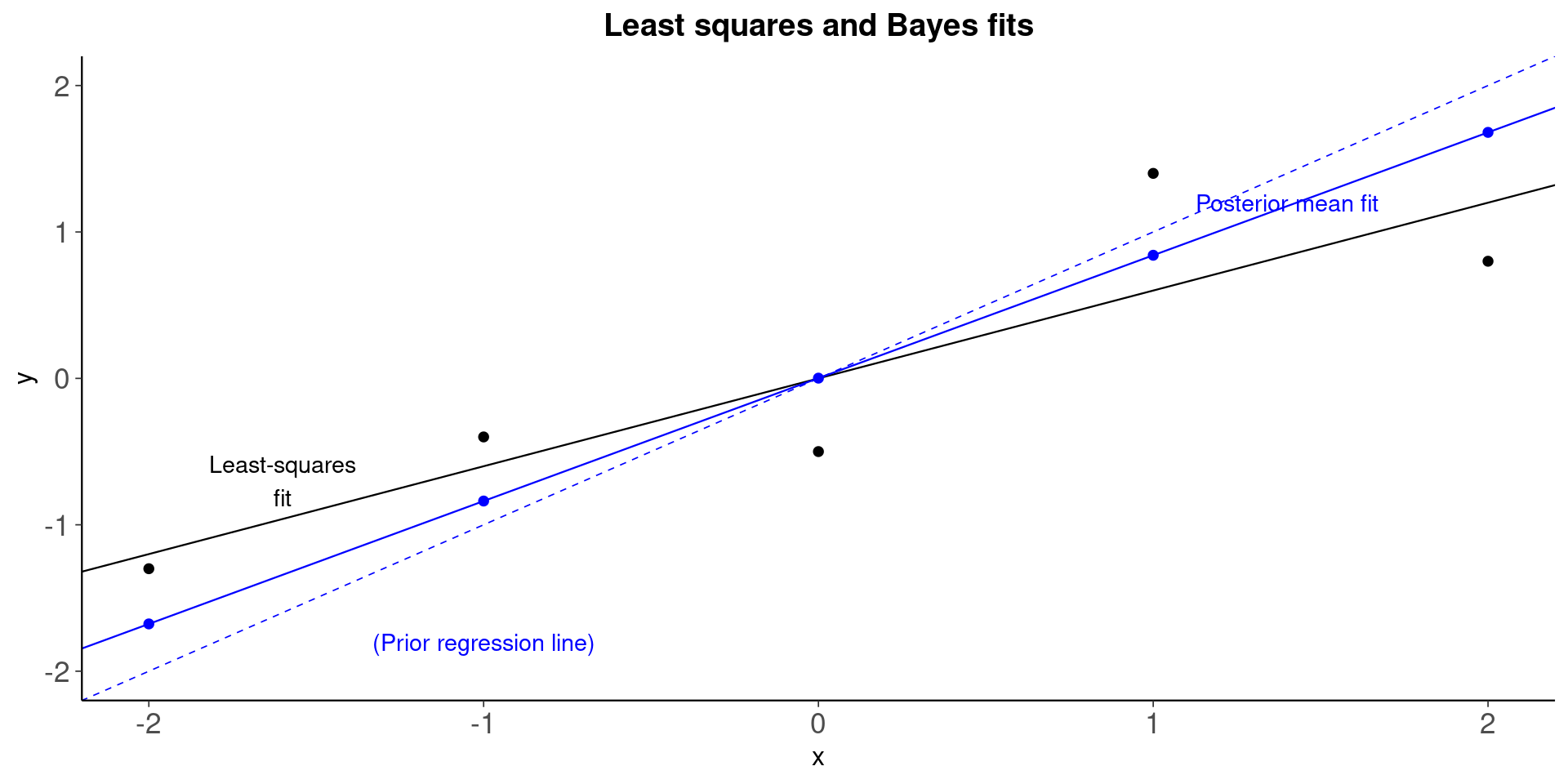

fig_1b <-
  ggplot(xy, aes(x, y)) +
  geom_abline( # 20 posterior draws of the regression line
    intercept = samp_20_draws[, 1],
    slope = samp_20_draws[, 2],
    color = "#9497eb",
    size = 0.25
  ) +
  geom_abline( # posterior mean regression line
    intercept = post_means[1],
    slope = post_means[2],
    color = "#1c35c4",
    size = 1
  ) +
  geom_point() +
  ylim(range(x)) + 
  ggtitle("Bayes posterior simulations")
plot(fig_1b)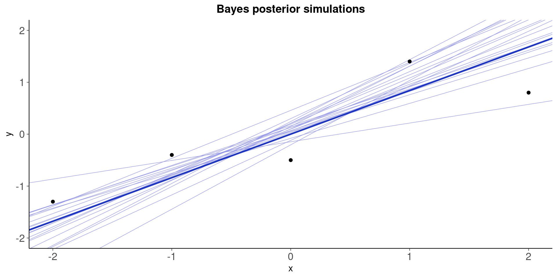

Bayesian R^2 Posterior and median

mcmc_hist(data.frame(bayesR2), binwidth=0.02)+xlim(c(0,1))+
  xlab(TeX('$R^2$'))+
  geom_vline(xintercept=median(bayesR2))+
  ggtitle('Bayesian R squared posterior and median')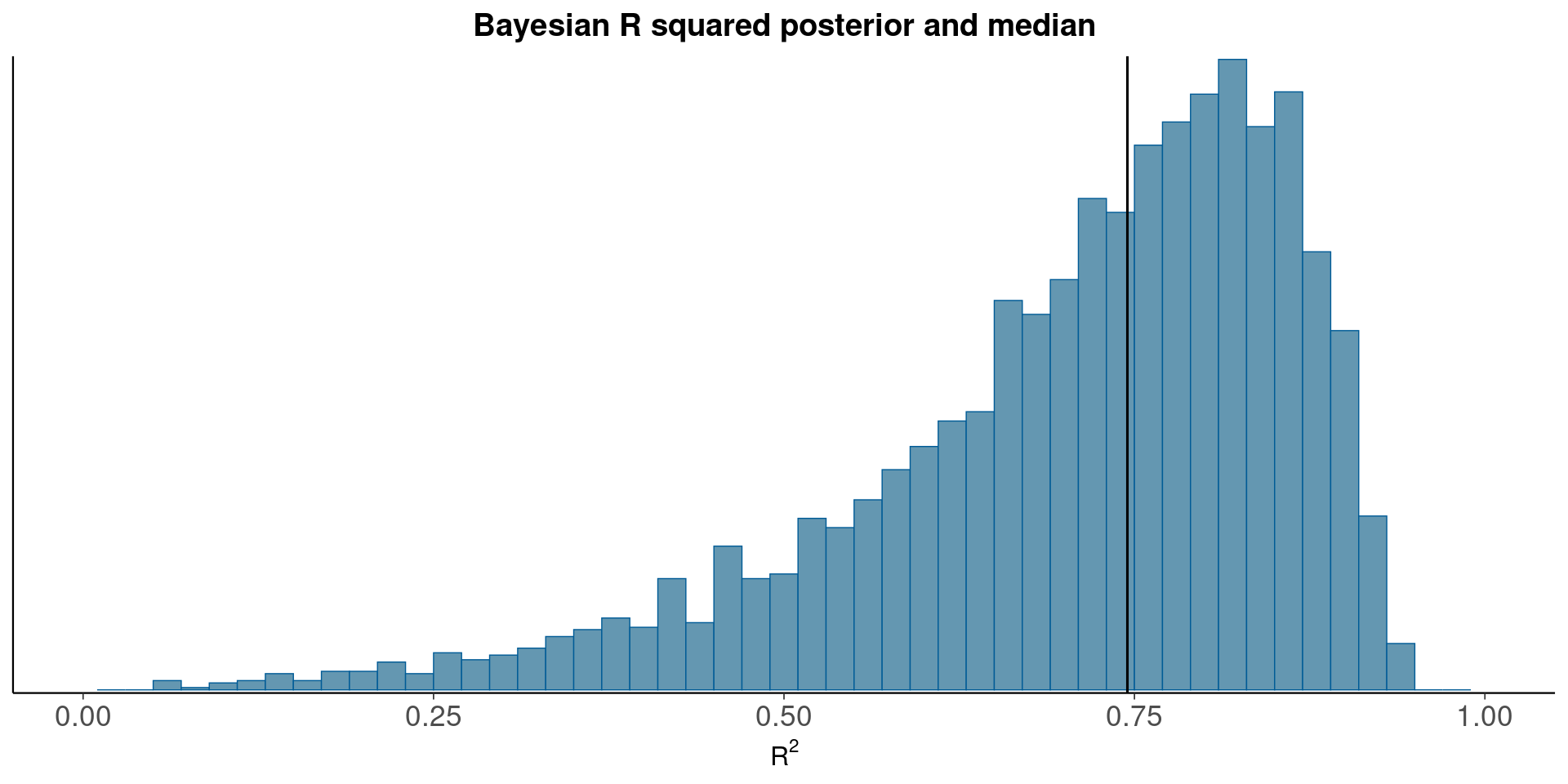

Compare draws from residual variances and sigma

fit<-fit_bayes
y <- rstanarm::get_y(fit)
ypred <- rstanarm::posterior_epred(fit)
e <- -1 * sweep(ypred, 2, y)
var_e <- apply(e, 1, var)
sigma <- as.matrix(fit, pars = c("sigma"))
qplot(sqrt(var_e),sigma)+geom_abline()+
    ggtitle('Toy data with n=5')+
    xlab('Draws from residual sd')+
    ylab('Draws from sigma')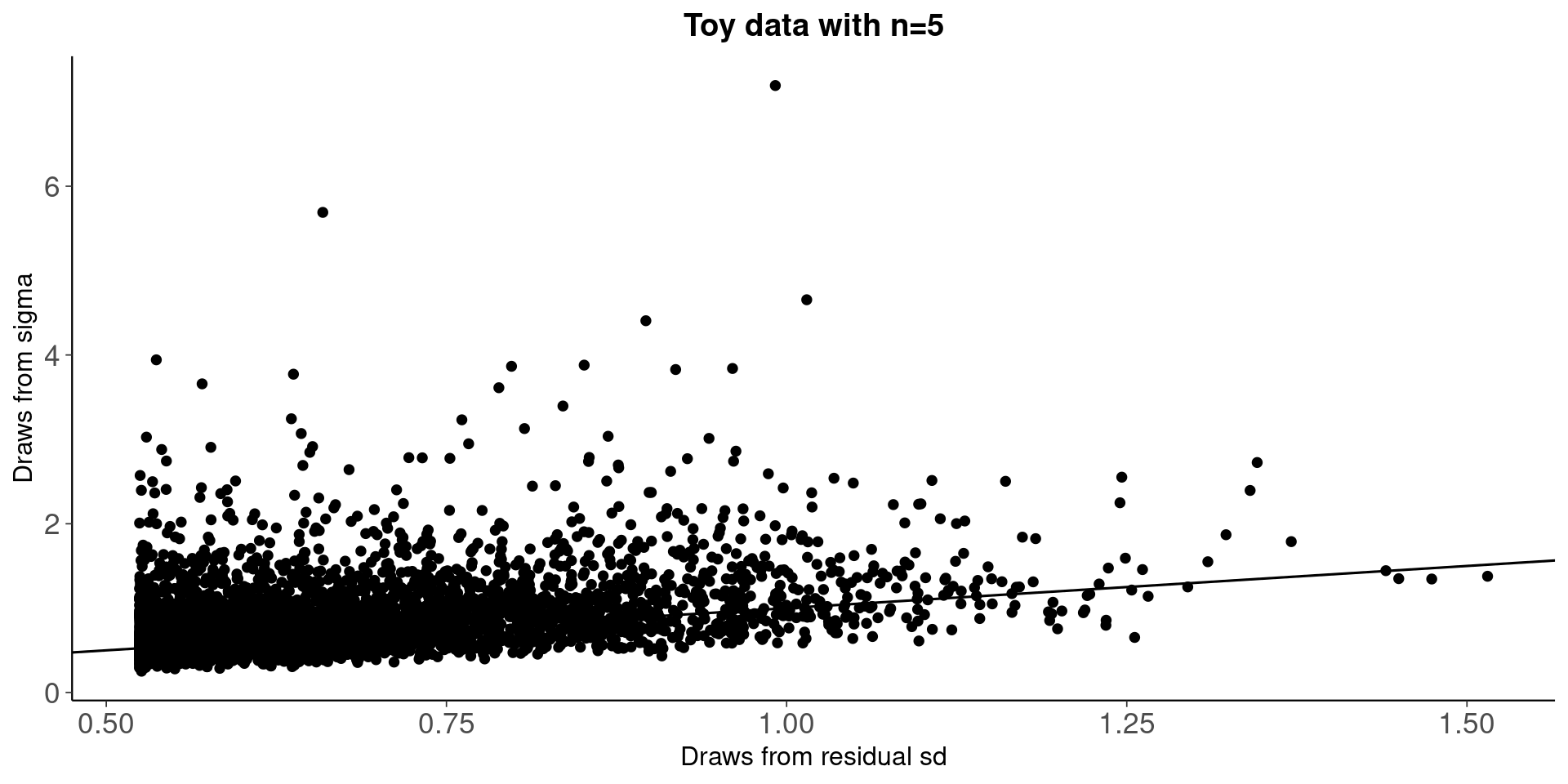

Draws from residual sd are truncated and not properly using the model information, which is reflected in R2 distribution below.

qplot(bayes_R2_res(fit_bayes),bayes_R2(fit_bayes))+geom_abline()+
    ggtitle('Toy data with n=5')+
    xlab('Bayesian R2 with draws from residual variance')+
    ylab('Bayesian R2 with draws from sigma')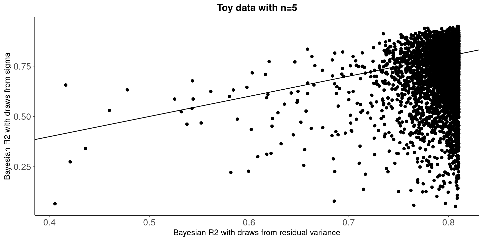

Compare residual and model based Bayesian R2, and Bayesian LOO-R2

pxl<-xlim(-0.5,1)
p1<-mcmc_hist(data.frame(bayesR2res), binwidth=0.02)+pxl+
    ggtitle('Toy data with n=5')+
    xlab('Bayesian R2 with draws from residuals')+
    geom_vline(xintercept=median(bayesR2res))
p2<-mcmc_hist(data.frame(bayesR2), binwidth=0.02)+pxl+
    xlab('Bayesian R2 with draws from sigma')+
    geom_vline(xintercept=median(bayesR2))
p3<-mcmc_hist(data.frame(looR2), binwidth=0.02)+pxl+
  xlab('Bayesian LOO-R2')+
  geom_vline(xintercept=median(looR2))
bayesplot_grid(p1,p2,p3)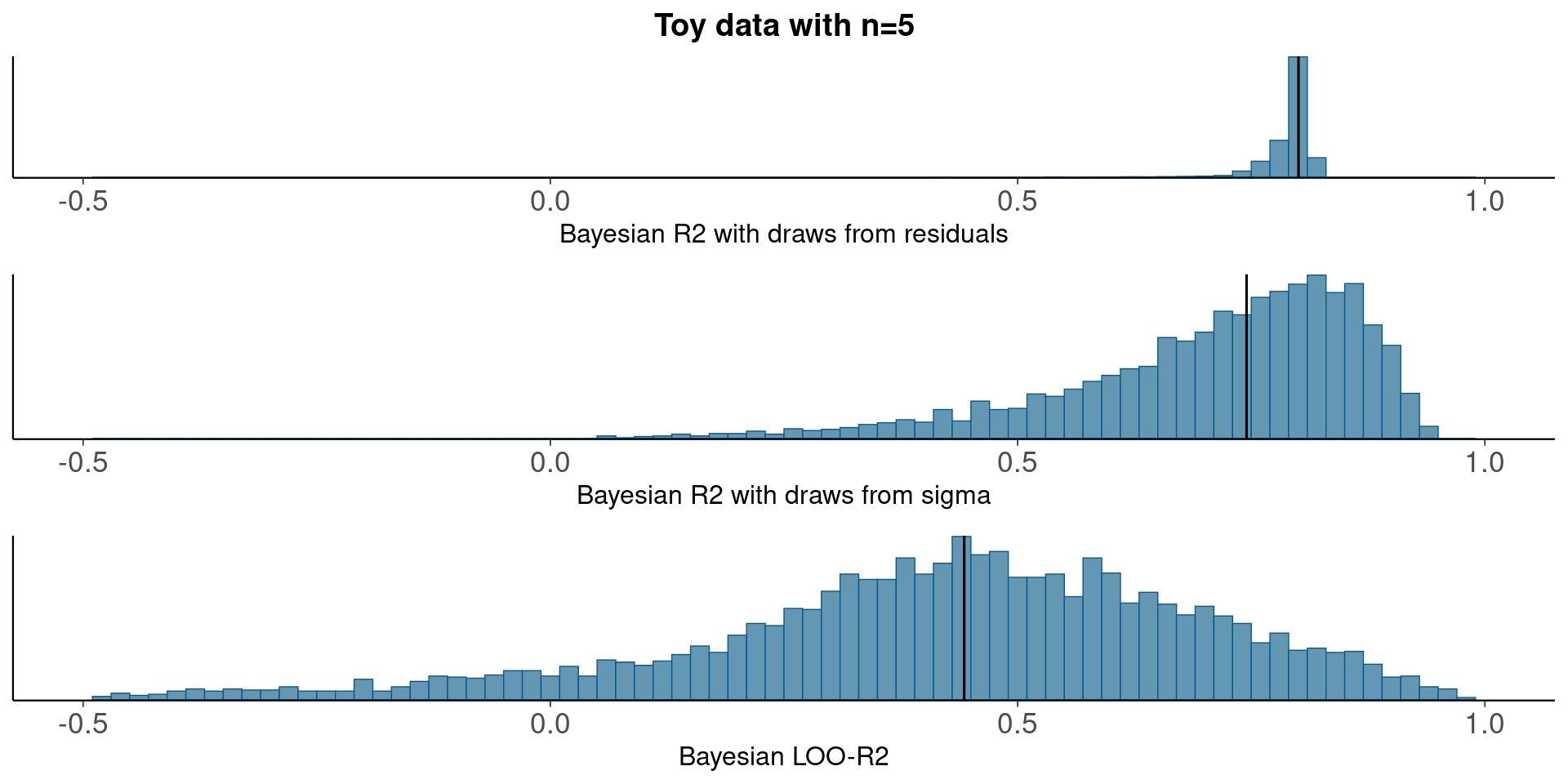

With small n, draws from the residual variance are not a good representation of the uncertainty.

3.2 Toy logistic regression example, n=20

set.seed(20)
y<-rbinom(n=20,size=1,prob=(1:20-0.5)/20)
data <- data.frame(rvote=y, income=1:20)

fit_logit <- stan_glm(rvote ~ income, family=binomial(link="logit"), data=data,
                      refresh=0)

Median Bayesian R2

round(median(bayesR2res<-bayes_R2_res(fit_logit)), 2)

[1] 0.36

round(median(bayesR2<-bayes_R2(fit_logit)), 2)

[1] 0.38

LOO-R2

looR2<-loo_R2(fit_logit)

Warning: Some Pareto k diagnostic values are slightly high. See help('pareto-k-diagnostic') for details.

round(median(looR2), 2)

[1] 0.3

With small n LOO-R2 is much lower than median of Bayesian R2

Compare residual and model based Bayesian R2, and Bayesian LOO-R2

pxl<-xlim(-.5,1)
p1<-mcmc_hist(data.frame(bayesR2res), binwidth=0.05)+pxl+
    ggtitle('Toy logistic data with n=20')+
    xlab('Bayesian R2 with draws from residuals')+
    geom_vline(xintercept=median(bayesR2res))
p2<-mcmc_hist(data.frame(bayesR2), binwidth=0.05)+pxl+
    xlab('Bayesian R2 with draws from sigma')+
    geom_vline(xintercept=median(bayesR2))
p3<-mcmc_hist(data.frame(looR2), binwidth=0.05)+pxl+
  xlab('Bayesian LOO-R2')+
  geom_vline(xintercept=median(looR2))
bayesplot_grid(p1,p2,p3)

With small n, draws from the residual variance are not a good representation of the uncertainty.

3.3 Mesquite - linear regression

Predicting the yields of mesquite bushes, n=46

Prepare data

head(mesquite)

  obs group diam1 diam2 total_height canopy_height density weight
1   1   MCD   1.8  1.15         1.30          1.00       1  401.3
2   2   MCD   1.7  1.35         1.35          1.33       1  513.7
3   3   MCD   2.8  2.55         2.16          0.60       1 1179.2
4   4   MCD   1.3  0.85         1.80          1.20       1  308.0
5   5   MCD   3.3  1.90         1.55          1.05       1  855.2
6   6   MCD   1.4  1.40         1.20          1.00       1  268.7

mesquite$canopy_volume <- mesquite$diam1 * mesquite$diam2 * mesquite$canopy_height
mesquite$canopy_area <- mesquite$diam1 * mesquite$diam2
mesquite$canopy_shape <- mesquite$diam1 / mesquite$diam2
(n <- nrow(mesquite))

[1] 46

Predict log weight model with log canopy volume, log canopy shape, and group

fit_5 <- stan_glm(log(weight) ~ log(canopy_volume) + log(canopy_shape) + group,
                  data=mesquite, refresh=0)

Median Bayesian R2

round(median(bayesR2res<-bayes_R2_res(fit_5)), 2)

[1] 0.87

round(median(bayesR2<-bayes_R2(fit_5)), 2)

[1] 0.87

LOO-R2

looR2<-loo_R2(fit_5)

Warning: Some Pareto k diagnostic values are slightly high. See help('pareto-k-diagnostic') for details.

round(median(looR2), 2)

[1] 0.86

LOO-R2 is slightly lower than median of Bayesian R2

Compare residual and model based Bayesian R2

pxl<-xlim(0.6, 0.95)
p1<-mcmc_hist(data.frame(bayesR2res), binwidth=0.01)+pxl+
    ggtitle('Mesquite data with n=46')+
    xlab('Bayesian R2 with draws from residuals')+
    geom_vline(xintercept=median(bayesR2res))
p2<-mcmc_hist(data.frame(bayesR2), binwidth=0.01)+pxl+
    xlab('Bayesian R2 with draws from sigma')+
    geom_vline(xintercept=median(bayesR2))
p3<-mcmc_hist(data.frame(looR2), binwidth=0.01)+pxl+
  xlab('Bayesian LOO-R2')+
  geom_vline(xintercept=median(looR2))
bayesplot_grid(p1,p2,p3)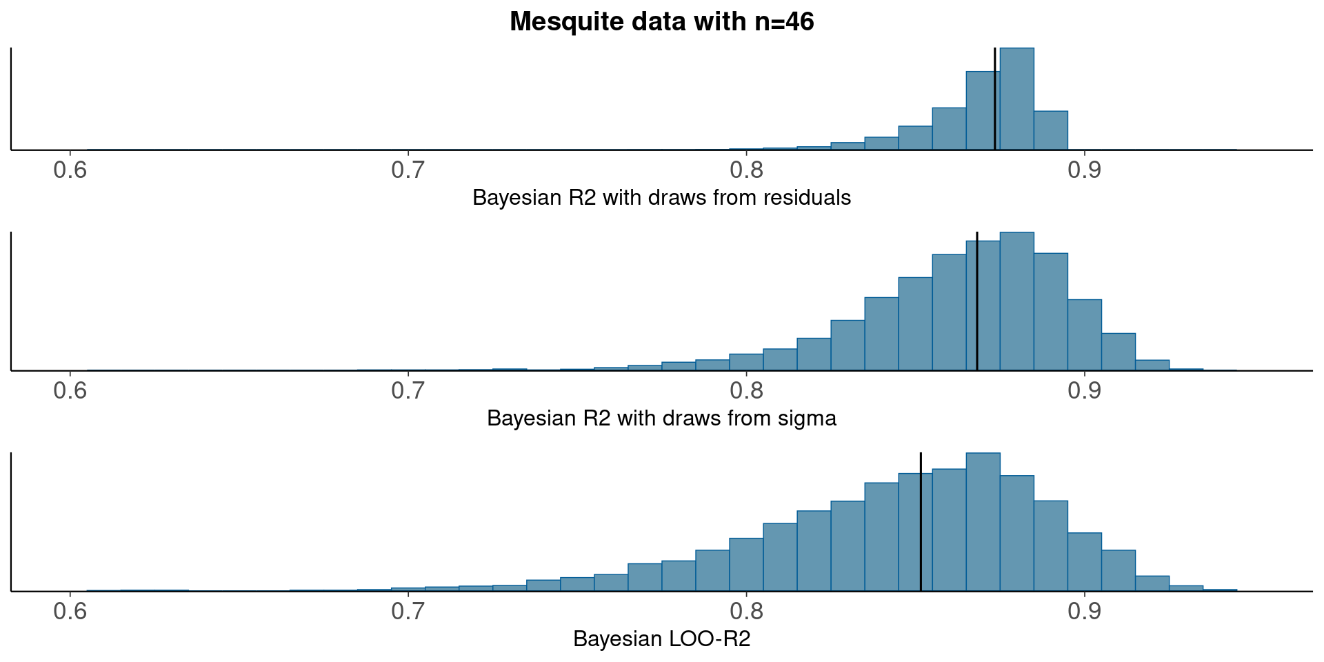

With small n, draws from the residual variance are not a good representation of the uncertainty and R2 distribution is more narrow (50%) than when using draws from the model sigma.

3.4 LowBwt – logistic regression

Predict low birth weight, n=189, from Hosmer and Lemeshow (2000)
This data was also used by Tjur (2009).

Prepare data

head(lowbwt)

  ID low age lwt race smoke ptl ht ui ftv  bwt
1 85   0  19 182    2     0   0  0  1   0 2523
2 86   0  33 155    3     0   0  0  0   3 2551
3 87   0  20 105    1     1   0  0  0   1 2557
4 88   0  21 108    1     1   0  0  1   2 2594
5 89   0  18 107    1     1   0  0  1   0 2600
6 91   0  21 124    3     0   0  0  0   0 2622

lowbwt$race <- factor(lowbwt$race)
(n <- nrow(lowbwt))

[1] 189

Predict low birth weight

fit <- stan_glm(low ~ age + lwt + race + smoke,
                family=binomial(link="logit"), data=lowbwt, refresh=0)

Median Bayesian R2

round(median(bayesR2res<-bayes_R2_res(fit)), 2)

[1] 0.12

round(median(bayesR2<-bayes_R2(fit)), 2)

[1] 0.12

LOO-R2

looR2<-loo_R2(fit)
round(median(looR2), 2)

[1] 0.03

LOO-R2 is much lower than median of Bayesian R2

Compare residual and model based Bayesian R2

pxl<-xlim(-0.15, 0.3)
p1<-mcmc_hist(data.frame(bayesR2res), binwidth=0.01)+pxl+
    ggtitle('Low birth weight data with n=189')+
    xlab('Bayesian R2 with draws from residuals')+
    geom_vline(xintercept=median(bayesR2res))
p2<-mcmc_hist(data.frame(bayesR2), binwidth=0.01)+pxl+
    xlab('Bayesian R2 with draws from sigma')+
    geom_vline(xintercept=median(bayesR2))
p3<-mcmc_hist(data.frame(looR2), binwidth=0.01)+pxl+
  xlab('Bayesian LOO-R2')+
  geom_vline(xintercept=median(looR2))
bayesplot_grid(p1,p2,p3)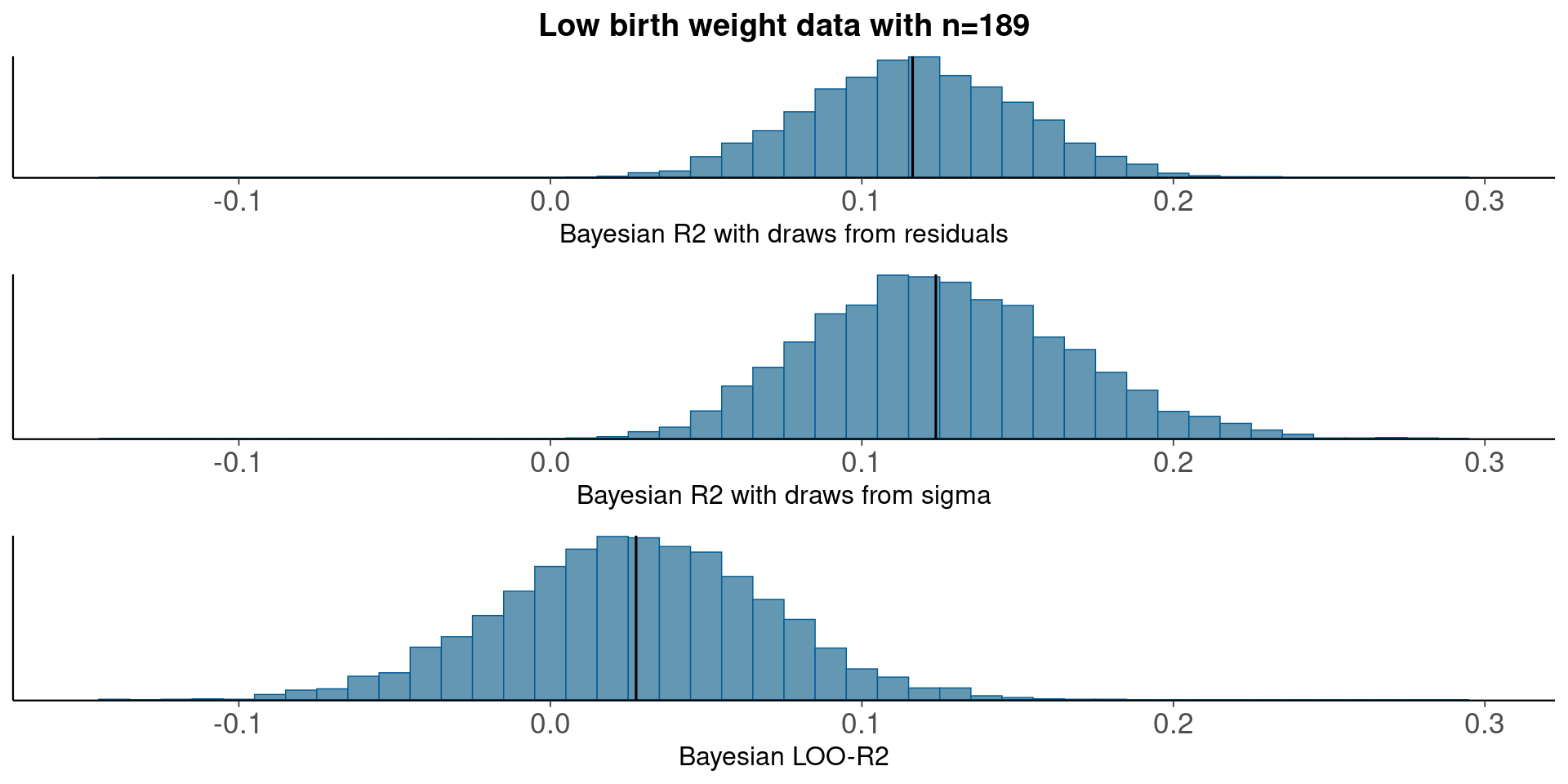

With moderate n, the distribution obtained using draws from the residual variances is still more narrow than the distribution obtained using draws from the model based variance.

3.5 LowBwt – linear regression

Predict birth weight, n=189, from Hosmer and Lemeshow (2000).
Tjur (2009) used logistic regression for dichotomized birth weight.
Below we use the continuos valued birth weight.

Predict birth weight

fit <- stan_glm(bwt ~ age + lwt + race + smoke, data=lowbwt, refresh=0)

Median Bayesian R2

round(median(bayesR2res<-bayes_R2_res(fit)), 2)

[1] 0.16

round(median(bayesR2<-bayes_R2(fit)), 2)

[1] 0.16

LOO-R2

looR2<-loo_R2(fit)
round(median(looR2), 2)

[1] 0.09

LOO-R2 is much lower than median of Bayesian R2

Compare residual and model based Bayesian R2

pxl<-xlim(-0.12, 0.36)
p1<-mcmc_hist(data.frame(bayesR2res), binwidth=0.01)+pxl+
    ggtitle('Birth weight data with n=189')+
    xlab('Bayesian R2 with draws from residuals')+
    geom_vline(xintercept=median(bayesR2res))
p2<-mcmc_hist(data.frame(bayesR2), binwidth=0.01)+pxl+
    xlab('Bayesian R2 with draws from sigma')+
    geom_vline(xintercept=median(bayesR2))
p3<-mcmc_hist(data.frame(looR2), binwidth=0.01)+pxl+
  xlab('Bayesian LOO-R2')+
  geom_vline(xintercept=median(looR2))
bayesplot_grid(p1,p2,p3)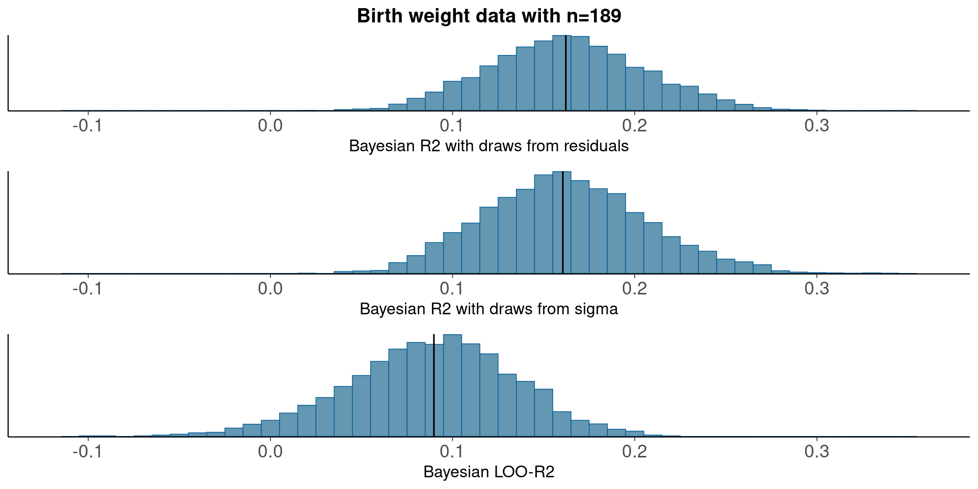

With moderate n, the distribution obtained using draws from the residual variances is still more narrow than the distribution obtained using draws from the model based variance.

3.6 KidIQ - linear regression

Children’s test scores data, n=434

Prepare data

head(kidiq)

  kid_score mom_hs    mom_iq mom_work mom_age
1        65      1 121.11753        4      27
2        98      1  89.36188        4      25
3        85      1 115.44316        4      27
4        83      1  99.44964        3      25
5       115      1  92.74571        4      27
6        98      0 107.90184        1      18

(n <- nrow(kidiq))

[1] 434

Predict test score

fit_3 <- stan_glm(kid_score ~ mom_hs + mom_iq, data=kidiq,
                  seed=1507, refresh=0)

Median Bayesian R2

round(median(bayesR2res<-bayes_R2_res(fit_3)), 2)

[1] 0.22

round(median(bayesR2<-bayes_R2(fit_3)), 2)

[1] 0.21

LOO-R2

looR2<-loo_R2(fit_3)
round(median(looR2), 2)

[1] 0.2

LOO-R2 is slightly lower than median of Bayesian R2

Compare residual and model based Bayesian R2

pxl<-xlim(0.05, 0.35)
p1<-mcmc_hist(data.frame(bayesR2res), binwidth=0.01)+pxl+
    ggtitle('KidIQ data with n=434')+
    xlab('Bayesian R2 with draws from residuals')+
    geom_vline(xintercept=median(bayesR2res))
p2<-mcmc_hist(data.frame(bayesR2), binwidth=0.01)+pxl+
    xlab('Bayesian R2 with draws from sigma')+
    geom_vline(xintercept=median(bayesR2))
p3<-mcmc_hist(data.frame(looR2), binwidth=0.01)+pxl+
  xlab('Bayesian LOO-R2')+
  geom_vline(xintercept=median(looR2))
bayesplot_grid(p1,p2,p3)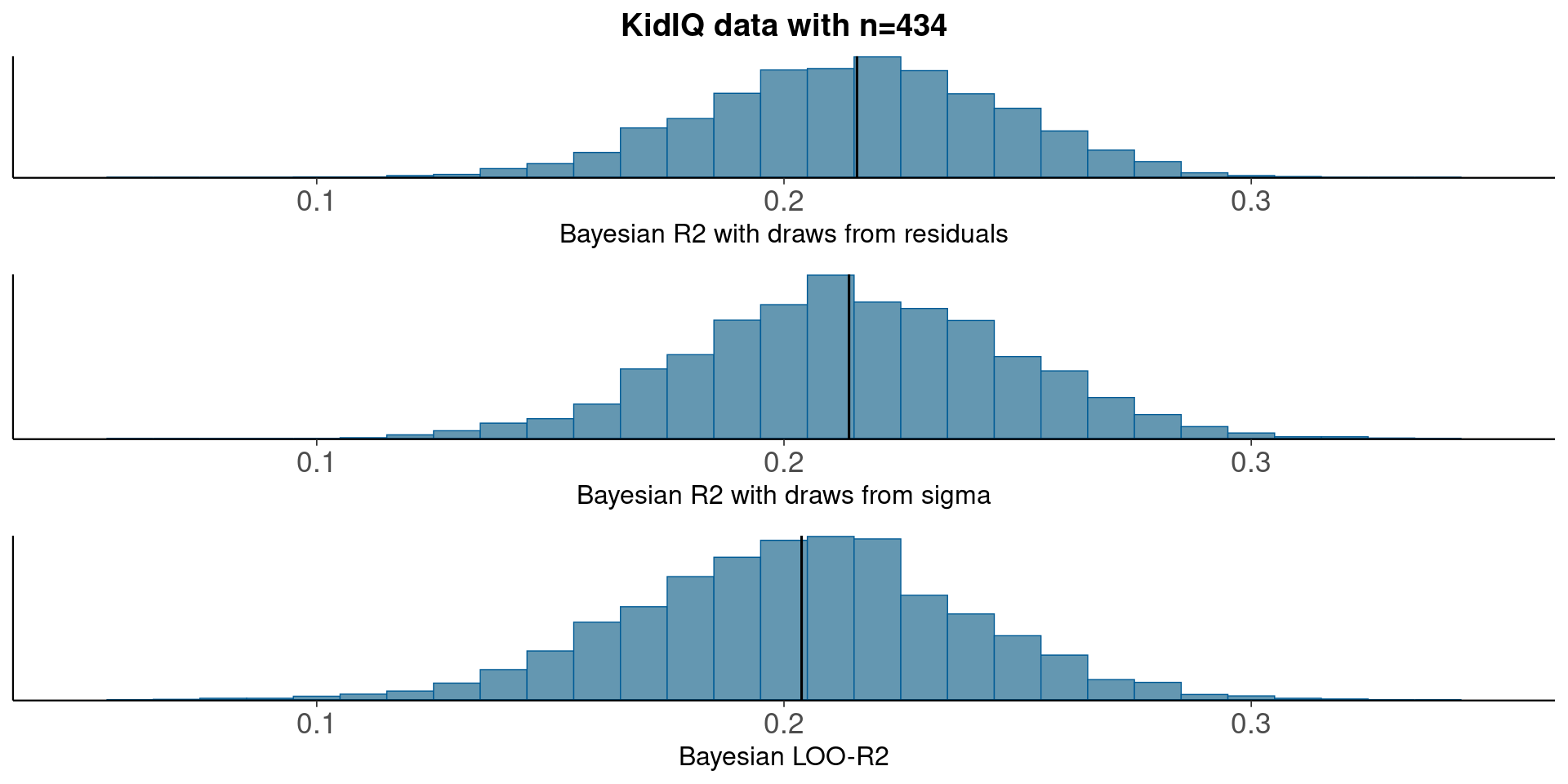

3.7 Earnings - logistic and linear regression

Predict respondents’ yearly earnings using survey data from 1990.
logistic regression n=1374, linear regression n=1187

Prepare data

head(earnings)

  height weight male  earn earnk ethnicity education mother_education father_education walk
1     74    210    1 50000    50     White        16               16               16    3
2     66    125    0 60000    60     White        16               16               16    6
3     64    126    0 30000    30     White        16               16               16    8
4     65    200    0 25000    25     White        17               17               NA    8
5     63    110    0 50000    50     Other        16               16               16    5
6     68    165    0 62000    62     Black        18               18               18    1
  exercise smokenow tense angry age
1        3        2     0     0  45
2        5        1     0     0  58
3        1        2     1     1  29
4        1        2     0     0  57
5        6        2     0     0  91
6        1        2     2     2  54

earnings_all <- earnings
earnings_all$positive <- earnings_all$earn > 0
(n_all <- nrow(earnings_all))

[1] 1816

# only non-zero earnings
earnings <- earnings_all[earnings_all$positive, ]
(n <- nrow(earnings))

[1] 1629

earnings$log_earn <- log(earnings$earn)
earnings_all$positive <- as.numeric(earnings_all$positive)

Bayesian logistic regression on non-zero earnings
Null model

fit_0 <- stan_glm(positive ~ 1, family = binomial(link = "logit"),
                  data = earnings_all, refresh=0)

loo0<-loo(fit_0)

Predict using height and sex

fit_1a <- stan_glm(positive ~ height + male, family = binomial(link = "logit"),
                   data = earnings_all, refresh=0)

loo1a<-loo(fit_1a)
loo_compare(loo0, loo1a)

       elpd_diff se_diff
fit_1a   0.0       0.0  
fit_0  -47.2       8.6

There is a clear difference in predictive performance.

Median Bayesian R2

round(median(bayesR2res<-bayes_R2_res(fit_1a)), 3)

[1] 0.046

round(median(bayesR2<-bayes_R2(fit_1a)), 3)

[1] 0.046

LOO-R2

looR2<-loo_R2(fit_1a)
round(median(looR2), 2)

[1] 0.04

LOO-R2 is slightly lower than median of Bayesian R2

Compare residual and model based Bayesian R2

pxl<-xlim(0.02, 0.11)
p1<-mcmc_hist(data.frame(bayesR2res), binwidth=0.002)+pxl+
    ggtitle('Earnings data with n=1374')+
    xlab('Bayesian R2 with draws from residuals')+
    geom_vline(xintercept=median(bayesR2res))
p2<-mcmc_hist(data.frame(bayesR2), binwidth=0.002)+pxl+
    xlab('Bayesian R2 with draws from sigma')+
    geom_vline(xintercept=median(bayesR2))
p3<-mcmc_hist(data.frame(looR2), binwidth=0.002)+pxl+
  xlab('Bayesian LOO-R2')+
  geom_vline(xintercept=median(looR2))
bayesplot_grid(p1,p2,p3)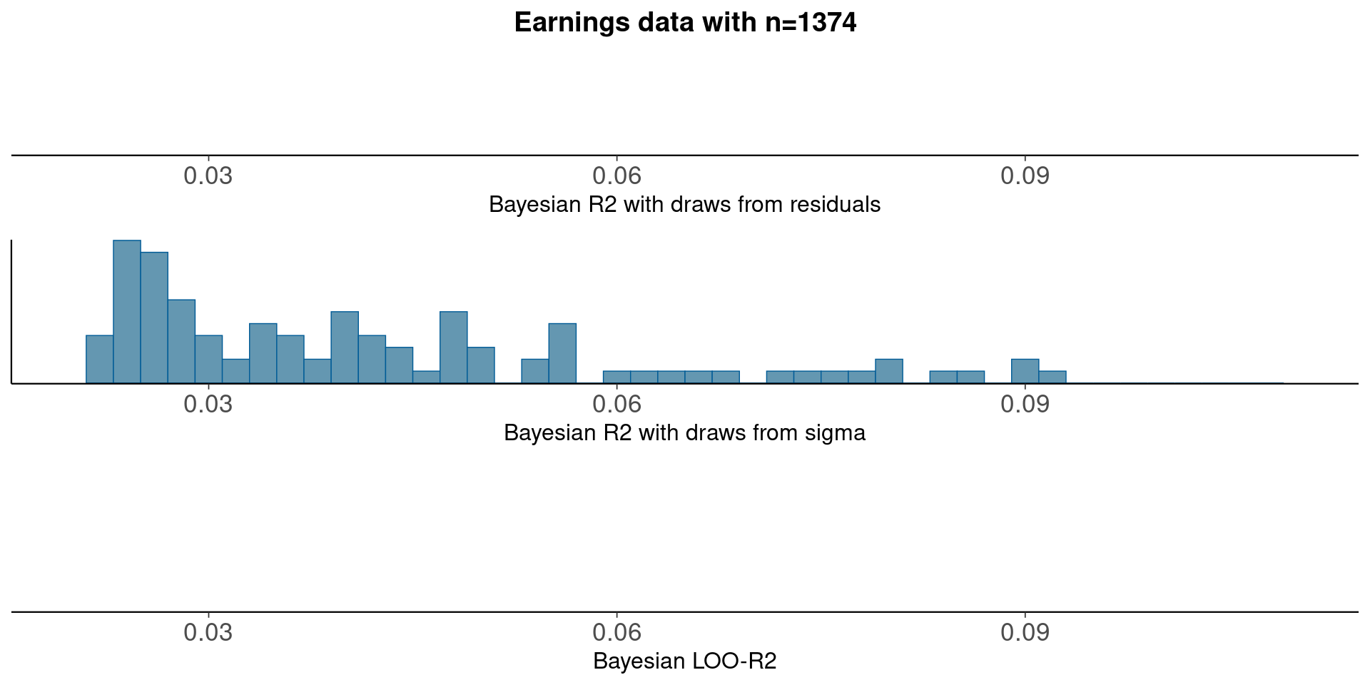

With plenty of data, there is not much difference between using draws from residuals or from sigma.

Bayesian probit regression on non-zero earnings

fit_1p <- stan_glm(positive ~ height + male,
                   family = binomial(link = "probit"),
                   data = earnings_all, refresh=0)

loo1p<-loo(fit_1p)
loo_compare(loo1a, loo1p)

       elpd_diff se_diff
fit_1p 0.0       0.0    
fit_1a 0.0       0.2

There is no practical difference in predictive performance between logit and probit.

Median Bayesian R2

round(median(bayesR2), 3)

[1] 0.046

round(median(bayesR2p<-bayes_R2(fit_1p)), 3)

[1] 0.046

LOO-R2

looR2p<-loo_R2(fit_1p)
round(median(looR2), 2)

[1] 0.04

round(median(looR2p), 2)

[1] 0.04

LOO-R2 is slightly lower than median of Bayesian R2

Compare logistic and probit models using new Bayesian R2

pxl<-xlim(0.02, 0.11)
p1<-mcmc_hist(data.frame(bayesR2), binwidth=0.002)+pxl+
    ggtitle('Earnings data with n=1374')+
    xlab('Bayesian R2 for logistic model')+
    geom_vline(xintercept=median(bayesR2))
p2<-mcmc_hist(data.frame(bayesR2p), binwidth=0.002)+pxl+
    xlab('Bayesian R2 for probit model')+
    geom_vline(xintercept=median(bayesR2p))
p3<-mcmc_hist(data.frame(looR2), binwidth=0.002)+pxl+
  xlab('Bayesian LOO-R2 for logistic model')+
  geom_vline(xintercept=median(looR2))
p4<-mcmc_hist(data.frame(looR2p), binwidth=0.002)+pxl+
  xlab('Bayesian LOO-R2 for probit model')+
  geom_vline(xintercept=median(looR2p))
bayesplot_grid(p1,p3,p2,p4)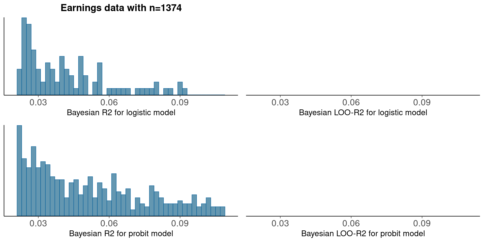

There is no practical difference in predictive performance between logit and probit.

Bayesian model on positive earnings on log scale

fit_1b <- stan_glm(log_earn ~ height + male, data = earnings, refresh=0)

Median Bayesian R2

round(median(bayesR2res<-bayes_R2_res(fit_1b)), 3)

[1] 0.081

round(median(bayesR2<-bayes_R2(fit_1b)), 3)

[1] 0.08

LOO-R2

looR2<-loo_R2(fit_1b)
round(median(looR2), 2)

[1] 0.08

LOO-R2 is slightly lower than median of Bayesian R2

Compare residual and model based Bayesian R2

pxl<-xlim(0.02, 0.15)
p1<-mcmc_hist(data.frame(bayesR2res), binwidth=0.002)+pxl+
    ggtitle('Positive earnings data with n=1187')+
    xlab('Bayesian R2 with draws from residuals')+
    geom_vline(xintercept=median(bayesR2res))
p2<-mcmc_hist(data.frame(bayesR2), binwidth=0.002)+pxl+
    xlab('Bayesian R2 with draws from sigma')+
    geom_vline(xintercept=median(bayesR2))
p3<-mcmc_hist(data.frame(looR2), binwidth=0.002)+pxl+
  xlab('Bayesian LOO-R2')+
  geom_vline(xintercept=median(looR2))
bayesplot_grid(p1,p2,p3)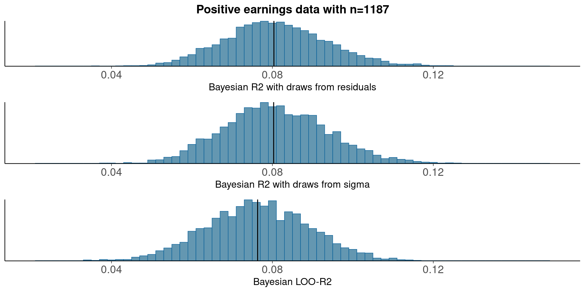

With plenty of data, there is not much difference between using draws from residuals or from sigma.

References

Hosmer, D. W. and Lemeshow, S. (2000) Applied logistic regression. Wiley.

Tjur, T. (2009) ‘Coefficient of determination in logistic regression models—A new proposal: The coefficient of discrimination’, American Statistician, 63, pp. 366–372.

Vehtari, A. and Lampinen, J. (2002) ‘Bayesian model assessment and comparison using cross-validation predictive densities’, Neural Computation, 14(10), pp. 2439–2468.

Vehtari, A. and Ojanen, J. (2012) ‘A survey of Bayesian predictive methods for model assessment, selection and comparison’, Statistics Surveys, 6, pp. 142–228.

Bayesian R2 and LOO-R2

Aki Vehtari, Andrew Gelman, Ben Goodrich, Jonah Gabry

First version 2019-01-02. Last modified 2022-02-21

1 Introduction

2 Functions for Bayesian R-squared for stan_glm models.

3 Experiments

3.1 Toy data with n=5

3.2 Toy logistic regression example, n=20

3.3 Mesquite - linear regression

3.4 LowBwt – logistic regression

3.5 LowBwt – linear regression

3.6 KidIQ - linear regression

3.7 Earnings - logistic and linear regression

References