Assignment set:
assignment1: Bayesian Data Analysis: Assignment 1
The assignment contain the following (3) tasks:
- p_red
- p_box
- p_identical_twinNotebook for Assignment 1
1 General information
The exercises here refer to the lecture 1/BDA chapter 1 content, not the course infrastructure quiz. This assignment is meant to test whether or not you have sufficient knowledge to participate in the course. The first question checks that you remember basic terms of probability calculus. The second exercise checks you recognise the most important notation used throughout the course and used in BDA3. The third-fifth exercise you will solve some basic Bayes theorem questions to check your understanding on the basics of probability theory. The 6th exercise checks on whether you recall the three steps of Bayesian Data Ananlysis as mentioned in chapter 1 of BDA3. The last exercise walks you through an example of how we can use models to generate distributions for outcomes of interest, applied to a setting of a simplified Roulette table.
This quarto document is not intended to be submitted, but to render the questions as they appear on Mycourses to be available also outside of it. The following will set-up markmyassignment to check your functions at the end of the notebook:
2 Bayes’ theorem 1
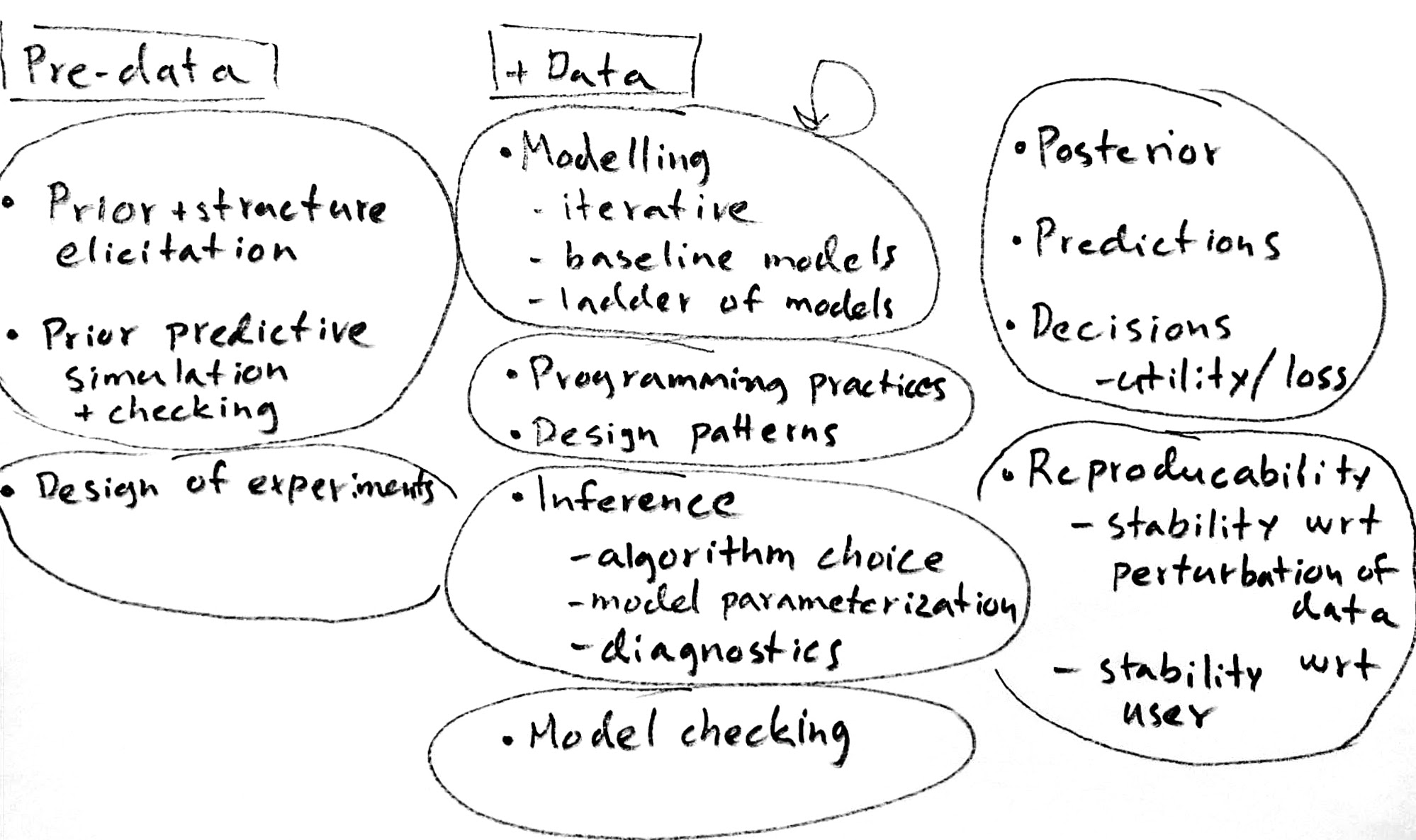
If you use pen and paper, it may help to draw pictures as follows (see also assignment_instructions#fig-workflow):

See Figure 1 for illustration of parts of Bayesian workflow.
3 Bayes’ theorem 2
The following will help you implementing a function to calculate the required probabilities for this exercise. Keep the below name and format for the function to work with markmyassignment:
boxes_test <- matrix(c(2,2,1,5,5,1), ncol = 2,
    dimnames = list(c("A", "B", "C"), c("red", "white")))

p_red <- function(boxes) {
    # Do computation here, and return as below.
    # This is the correct return value for the test data provided above.
    0.3928571
}

p_box <- function(boxes) {
    # Do computation here, and return as below.
    # This is the correct return value for the test data provided above.
    c(0.29090909,0.07272727,0.63636364)
}
4 A Binomial Model for the Roulette Table
Incomplete code can be found below.
# proportion of red/black
theta <- # declare probability parameter for the binomial model

# Sequence of trials

trials <- seq(#start value of sequence,#end value of sequence,#value for spacing)

# Number of simulation draws from the model
nsims <- # number of of simulations from the binomial model

# Helper function for getting the proportions
binom_gen <- function(trials,theta,nsims){
    df <-  as.data.frame(rbinom(nsims,trials,theta)/trials) |> mutate(nsims = nsims,trials = trials)
    colnames(df) <- c("Proportions","Nsims","Trials")
  return(df)
}

# Create a data frame containing the draws for each number of trials
proportion_60 <- do.call(rbind, lapply(trials, binom_gen, theta, nsims)) # lapply applies elements in trials column to binom_gen function, which is then rowbound via do.call
Now plot a histogram of the computed proportions for 10, 50 and 1000 trials, using the code below
Suppose you are now certain that theta = 0.6, plot the probability density given 1000 trials using the code below.
size =  # number of trials
prob =  # probability of success

binom_data <- data.frame(
  Success = 0:size,
  Probability = dbinom(0:size, size = size, prob = prob)
)

ggplot(binom_data, aes(x = Success, y = Probability)) +
  geom_point() +
  geom_line() +
labs(title = "PMF of Binomial Distribution", x = "Number of Successes", y = "PDF")The following will check the functions for which markmyassignment has been set up:
✔ | F W  S  OK | Context

⠏ |          0 | task-1-subtask-1-tests
⠏ |          0 | p_red()
✖ | 1        3 | p_red()
────────────────────────────────────────────────────────────────────────────────
Failure ('test-task-1-subtask-1-tests.R:21:3'): p_red()
Expected `p_red(boxes = boxes)` to be equivalent to 0.5.
1/1 mismatches
[1] 0.393 - 0.5 == -0.107
Error: Incorrect result for matrix(c(1,1,1,1,1,1), ncol = 2)
────────────────────────────────────────────────────────────────────────────────

⠏ |          0 | task-2-subtask-1-tests
⠏ |          0 | p_box()
✖ | 1        3 | p_box()
────────────────────────────────────────────────────────────────────────────────
Failure ('test-task-2-subtask-1-tests.R:19:3'): p_box()
Expected `p_box(boxes = boxes)` to be equivalent to `c(0.4, 0.1, 0.5)`.
3/3 mismatches (average diff: 0.0909)
[1] 0.2909 - 0.4 == -0.1091
[2] 0.0727 - 0.1 == -0.0273
[3] 0.6364 - 0.5 ==  0.1364
Error: Incorrect result for matrix(c(1,1,1,1,1,1), ncol = 2)
────────────────────────────────────────────────────────────────────────────────

⠏ |          0 | task-3-subtask-1-tests
⠏ |          0 | p_identical_twin()
⠙ | 2        0 | p_identical_twin()
✖ | 2        0 | p_identical_twin()
────────────────────────────────────────────────────────────────────────────────
Failure ('test-task-3-subtask-1-tests.R:8:3'): p_identical_twin()
Expected `exists("p_identical_twin")` to be TRUE.
Differences:
`actual`:   FALSE
`expected`: TRUE

Error: p_identical_twin() is missing

Error ('test-task-3-subtask-1-tests.R:10:3'): p_identical_twin()
Error in `eval(code, test_env)`: object 'p_identical_twin' not found
Backtrace:
    ▆
 1. └─checkmate::expect_function(...) at test-task-3-subtask-1-tests.R:10:3
 2.   └─checkmate::checkFunction(x, args, ordered, nargs, null.ok)
────────────────────────────────────────────────────────────────────────────────

══ Results ═════════════════════════════════════════════════════════════════════
── Failed tests ────────────────────────────────────────────────────────────────
Failure ('test-task-1-subtask-1-tests.R:21:3'): p_red()
Expected `p_red(boxes = boxes)` to be equivalent to 0.5.
1/1 mismatches
[1] 0.393 - 0.5 == -0.107
Error: Incorrect result for matrix(c(1,1,1,1,1,1), ncol = 2)

Failure ('test-task-2-subtask-1-tests.R:19:3'): p_box()
Expected `p_box(boxes = boxes)` to be equivalent to `c(0.4, 0.1, 0.5)`.
3/3 mismatches (average diff: 0.0909)
[1] 0.2909 - 0.4 == -0.1091
[2] 0.0727 - 0.1 == -0.0273
[3] 0.6364 - 0.5 ==  0.1364
Error: Incorrect result for matrix(c(1,1,1,1,1,1), ncol = 2)

Failure ('test-task-3-subtask-1-tests.R:8:3'): p_identical_twin()
Expected `exists("p_identical_twin")` to be TRUE.
Differences:
`actual`:   FALSE
`expected`: TRUE

Error: p_identical_twin() is missing

Error ('test-task-3-subtask-1-tests.R:10:3'): p_identical_twin()
Error in `eval(code, test_env)`: object 'p_identical_twin' not found
Backtrace:
    ▆
 1. └─checkmate::expect_function(...) at test-task-3-subtask-1-tests.R:10:3
 2.   └─checkmate::checkFunction(x, args, ordered, nargs, null.ok)

[ FAIL 4 | WARN 0 | SKIP 0 | PASS 6 ]