---
title: "Notebook for Assignment 7"
author: "Aki Vehtari et al."
format:
html:
toc: true
code-tools: true
code-line-numbers: true
number-sections: true
mainfont: Georgia, serif
editor: source
---
# General information
This assignment relates to Lecture 7 and Chapter 5.
We recommend using [JupyterHub](https://jupyter.cs.aalto.fi) (which has all the needed packages pre-installed).
::: hint
**Reading instructions:**
- [**The reading instructions for BDA3 Chapter 5**](../BDA3_notes.html#ch5).
:::
{{< include includes/_general_cloze_instructions.md >}}
```{r}
if (!require(tidybayes)) {
    install.packages("tidybayes")
    library(tidybayes)
}
if (!require(brms)) {
    install.packages("brms")
    library(brms)
}
if(!require(ggplot2)) {
  install.packages("ggplot2")
  library(ggplot2)
}
if (!require(metadat)) {
  install.packages("metadat")
  library(metadat)
}
if(!require(cmdstanr)){
    install.packages("cmdstanr", repos = c("https://mc-stan.org/r-packages/", getOption("repos")))
    library(cmdstanr)
}
cmdstan_installed <- function(){
  res <- try(out <- cmdstanr::cmdstan_path(), silent = TRUE)
  !inherits(res, "try-error")
}
if(!cmdstan_installed()){
    install_cmdstan()
}
```
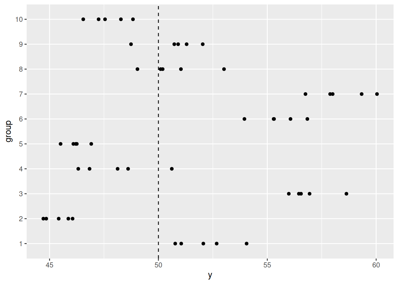
# Simulation warm-up
Here is the function to simulate and plot observations from a
hierarchical data-generating process.
```{r}
hierarchical_sim <- function(group_pop_mean,
                             between_group_sd,
                             within_group_sd,
                             n_groups,
                             n_obs_per_group
                             ) {
  # Generate group means
  group_means <- rnorm(
    n = n_groups,
    mean = group_pop_mean,
    sd = between_group_sd
  )

  # Generate observations

  ## Create an empty vector for observations
  y <- numeric()
  ## Create a vector for the group identifier
  group <- rep(1:n_groups, each = n_obs_per_group)

  for (j in 1:n_groups) {
    ### Generate one group observations
    group_y <- rnorm(
      n = n_obs_per_group,
      mean = group_means[j],
      sd = within_group_sd
    )
    ### Append the group observations to the vector
    y <- c(y, group_y)
  }

  # Combine into a data frame
  data <- data.frame(
    group = factor(group),
    y = y
  )

  # Plot the data
  ggplot(data, aes(x = y, y = group)) +
    geom_point() +
    geom_vline(xintercept = group_pop_mean, linetype = "dashed")
}
```
Example using the function:
```{r}
hierarchical_sim(
  group_pop_mean = 50,
  between_group_sd = 5,
  within_group_sd = 1,
  n_groups = 10,
  n_obs_per_group = 5
  )
```
# Sleep deprivation
The dataset `sleepstudy` is available by using the command
`data(sleepstudy, package = "lme4")`
Below is some code for fitting a brms model. This model is a simple
pooled model. You will need to fit a hierarchical model as explained
in the assignment, but this code should help getting started.
Load the dataset
```{r}
data(sleepstudy, package = "lme4")
```
Specify the formula and observation family:
```{r}
#| eval: false
sleepstudy_pooled_formula <- bf(
  Reaction ~ 1 + Days,
  family = "gaussian",
  center = FALSE
)
```
We can see the parameters and default priors with
```{r}
#| eval: false
get_prior(pooled_formula, data = sleepstudy)
```
We can then specify the priors:
```{r}
#| eval: false
(sleepstudy_pooled_priors <- c(
  prior(
    normal(400, 100),
    class = "b",
    coef = "Intercept"
  ),
  prior(
    normal(0, 50),
    class = "b",
    coef = "Days"
  ),
  prior(
    normal(0, 50),
    class = "sigma"
  )
))
```
And then fit the model:
```{r}
#| eval: false
sleepstudy_pooled_fit <- brm(
  formula = pooled_formula,
  prior = sleepstudy_pooled_priors,
  data = sleepstudy
)
```
We can inspect the model fit:
```{r}
#| eval: false
summary(pooled_fit)
```
To plot `conditional_effects`, you can do that as follows:
```{r}
#| eval: false
conditions <- make_conditions(sleepstudy, "Subject", incl_vars = FALSE)
me <- conditional_effects(sleepstudy_pooled_fit, conditions = conditions,
                          re_formula = NULL)
plot(me, ncol = 6, points = TRUE)
```
# School calendar
Meta-analysis models can be fit in brms. When the standard error is
known, the `se()` function can be used to specify it.
The dataset `dat.konstantopoulos2011` has the observations for the school calendar intervention meta-analysis.
```{r}
data(dat.konstantopoulos2011, package = "metadat")
```
As mentioned in the assignment instructions, a unique identifier for
school needs to be created by combining the district and school:
```{r}
#| eval: false
schoolcalendar_data <- dat.konstantopoulos2011 |>
  dplyr::mutate(
    school = factor(school),
    district = factor(district),
    district_school = interaction(district, school, drop = TRUE, sep = "_")
  )
```
Then the models can be fit
```{r}
#| eval: false
schoolcalendar_pooled_formula <- bf(
  formula = yi | se(sqrt(vi)) ~ 1,
  family = "gaussian"
)

schoolcalendar_pooled_fit <- brm(
  formula = schoolcalendar_pooled_formula,
  data = schoolcalendar_data
)
```
Predictions for a new school can be made using the `posterior_epred` function:
```{r}
#| eval: false
new_school <- data.frame(
  school = factor(1),
  district = factor(1),
  district_school = factor("1_1"),
  vi = 0 # the expectation of the prediction is not affected by the sampling variance, so this can be any number
)


schoolcalendar_post_epred <- posterior_epred(
    schoolcalendar_pooled_fit,
    newdata = new_school,
    allow_new_levels = TRUE
  )
```
It can be helpful to plot the posterior estimates. Here is a function that will do this:
```{r}
#| eval: false
plot_school_posteriors <- function(fit, dataset) {
  tidybayes::add_predicted_draws(dataset, fit) |>
    ggplot(
      aes(
        x = .prediction,
        y = interaction(district, school, sep = ", ", lex.order = TRUE))) +
    tidybayes::stat_halfeye() +
    ylab("District, school") +
    xlab("Posterior effect")
}
```
And can be used as follows:
```{r}
#| eval: false
plot_school_posteriors(
  fit = schoolcalendar_pooled_fit,
  dataset = schoolcalendar_data
)
```