Assignment 6
1 General information
The exercises here refer to the lecture 6/BDA chapter 12 content. The main topics for this assignment are the MCSE and importance sampling.
The exercises constitute 96% of the Quiz 6 grade.
We prepared a quarto notebook specific to this assignment to help you get started. You still need to fill in your answers on Mycourses! You can inspect this and future templates
- as a rendered html file (to access the qmd file click the “</> Code” button at the top right hand corner of the template)
- Questions below are exact copies of the text found in the MyCourses quiz and should serve as a notebook where you can store notes and code.
- We recommend opening these notebooks in the Aalto JupyterHub, see how to use R and RStudio remotely.
- For inspiration for code, have a look at the BDA R Demos and the specific Assignment code notebooks
- Recommended additional self study exercises for each chapter in BDA3 are listed in the course web page. These will help to gain deeper understanding of the topic.
- Common questions and answers regarding installation and technical problems can be found in Frequently Asked Questions (FAQ).
- Deadlines for all assignments can be found on the course web page and in MyCourses.
- You are allowed to discuss assignments with your friends, but it is not allowed to copy solutions directly from other students or from internet.
- Do not share your answers publicly.
- Do not copy answers from the internet or from previous years. We compare the answers to the answers from previous years and to the answers from other students this year.
- Use of AI is allowed on the course, but the most of the work needs to by the student, and you need to report whether you used AI and in which way you used them (See points 5 and 6 in Aalto guidelines for use of AI in teaching).
- All suspected plagiarism will be reported and investigated. See more about the Aalto University Code of Academic Integrity and Handling Violations Thereof.
- If you have any suggestions or improvements to the course material, please post in the course chat feedback channel, create an issue, or submit a pull request to the public repository!
- The decimal separator throughout the whole course is a dot, “.” (Follows English language convention). Please be aware that MyCourses will not accept numerical value answers with “,” as a decimal separator
- Unless stated otherwise: if the question instructions ask for reporting of numerical values in terms of the ith decimal digit, round to the ith decimal digit. For example, 0.0075 for two decimal digits should be reported as 0.01. More on this in Assignment 4.
1.1 Assignment questions
For convenience the assignment questions are copied below. Answer the questions in MyCourses.
Lecture 6/Chapter 12 of BDA Quiz (96% of grade)
This week’s assignment focuses on building the foundations for using frontier MCMC methods and the probabilistic programming language Stan. We will directly code in Stan, but later assignments will use the brms R package for building Stan models.
1. A brief overview of Hamiltonian Monte Carlo (HMC)
1.1 What is the intuition behind HMC as described in the course lectures?
In order to generate good proposals, HMC uses the Hamiltonian function and it’s partial derivatives to generate a path along the surface of the log posterior. As in the lecture, define \(\phi\) as the momentum variable which is of the same dimension as the parameter vector \(\theta\). The Hamiltonian function has two terms \(U(\theta)\) and \(K(\phi)\).
1.2 What is the intuition behind the term \(U(\theta)\)
1.3 What is the intuition behind the term \(K(\phi)\)
1.4 The partial derivatives of the Hamiltonian, also known as Hamilton’s equations, determine how \(\theta\) and \(\phi\) change during MCMC. What problem occurs when implementing Hamilton’s equations computationally?
1.5 All HMC implementations on a digital computer need to discretise the simulated trajectory dictated by Hamilton’s equations. Which computational method does Stan (and most other HMC-based algorithms) use for discretisation?
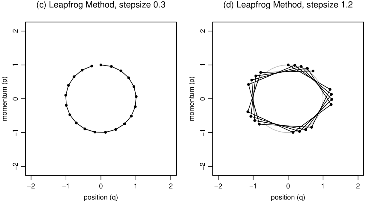
1.6 It is not necessary in this course to know the computational details behind the leapfrog integrator, only that it is applied for \(L\) steps along the Hamiltonian trajectory with step size, \(\epsilon\). The figure below by Neal (2012) shows dynamic simulation in the joint position-momentum space using leapfrog method. Based on these figures, which of the following statements is false?
HMC has two general steps at each iteration of the MCMC chain. Denote the current state of the MCMC chain as \(t\), then
- we draw a new momentum variable \(\phi\) (often assumed to distributed marginally Gaussian)
- perform a Metropolis update with \(r=\exp\left(-H(\theta^*,\phi^*)+H(\theta^{(t-1)},\phi^{(t-1)})\right)\), where Hamiltonian dynamics are used to produce the proposal. The two parameters of the algorithm, number of steps \(L\) and step size \(\epsilon\), need to be tuned.
1.7 What can happen eventually, when allowing the trajectory length, defined as step size times number of steps, \(\epsilon L\), to be long enough? Check out this interactive demo (algorithm=HamiltonianMC, target=standard) and set Leapfrog steps equal to 75 for visual intuition (if the demo freezes, close the demo, restart and instead of sliders, make the control changes by editing the values in the numeric fields). Do not adjust anything else in the demo.
To avoid this behaviour that static HMC with fixed integration time (number of steps times the step size) may have, the No-U-Turn (NUTS) algorithm by Hoffman and Gelman (2014) performs automatic tuning: neither the step size nor number of steps need be specified by the user. NUTS uses a tree-building algorithm (see the slides) to adaptively determine the number of steps, \(L\), while the step size is adapted during the warm-up phase according to a target average acceptance ratio. To gain some more intuition on the behaviour of the adaptivity of NUTS, open the interactive demo again with this link (algorithm=EfficientNUTS, target=banana). Set Autoplay delay to around 500, and set Leapfrog \(\delta t\) to 0.03. This algorithm corresponds to Algorithm 3 in Hoffman and Gelman (2014), where for a fixed \(\epsilon\), the algorithm adaptively determines the number of steps, \(L\).
1.8 What do you observe?
1.9 On the other hand, set Leapfrog \(\delta t\) to 0.6, all else equal. What do you observe?
The user does not need to select the stepsize directly. Stan includes also
adaptation of the step size in the warmup phase using stochastic optimization
called dual averaging. The user specifies a target acceptance ratio (in Stan
actually target for expected discretization error), with argument
adapt_delta, and a number of iterations during which adaptation
of \(\epsilon L\) occurs (warm-up draws).
Open, the interactive demo again with this link
(algorithm=DualAveragingNUTS, target=banana), and adjust the Autoplay delay to
around 70, but otherwise keep the default options, particularly, keep the
target acceptance ratio (here \(\delta\)) at
0.65. On the top left-hand corner m/M_adapt tells you how many draws have been
taken compared to number of warm-up draws. Wait until m/M_adapt is at least
50/200.
1.10 What do you observe with the first couple of iterations?
1.11 What do you observe with sufficient warm-up?
1.12 Now set the target acceptance ratio to 0.95. What do you observe?
1.13 Now set the target acceptance ratio to the smallest possible value. What do you observe?
The current Stan HMC-NUTS implementation has some further enhancements, but
we will not go to details of those. The main algorithm paramaters are
adapt_delta and max_treedepth options.
adapt_delta specifies the target expected discretization error
(in the same scale as the average proposal acceptance ratio), during the
warm-up phase. The default in most packages using Stan is
adapt_delta=0.8.
1.14 What should happen when you increase
adapt_delta, all else equal?
max_treedepth controls the maximum number of doublings in the
tree-building algorithm and thus controls the maximum number of steps in
Hamiltonian simulation. This allows the sampler to explore further away in the
distribution, which can be beneficial when dealing with complex posteriors.
The default in Stan is max_treedepth = 10.
1.15 What is the main cost to increasing the
max_treedepth?
1.16 Despite the adaptated step-size, you may encounter challenging posteriors, e.g. with highly varying curvature in log-density. What can happen if the step-size is too big compared to the curvature of the log-density?
2. Stan warmup
From 2018 to 2023, we have been keeping track of assignment submissions for the BDA course given the number of submissions for the 1st assignment. We will fit a simple linear model to answer two questions of interest:
- What is the trend of student retention as measured by assignment submissions?
- Given the submission rates for assignments 1-8, how many students will complete the final 9th assignment (and potentially pass the course)?
Below is broken Stan code for a linear model. In the following, we write the equations following the Stan distributional definitions. See Stan documentation for the definitions related to the normal distribution.
\(p(y \mid x, \alpha, \beta, \sigma) = \text{normal}(y \mid \alpha + \beta x, \sigma)\) (normal model)
\(p(\alpha, \beta, \sigma) \propto \text{const}\) (improper flat prior)
In both the statistical model above and in the Stan model below, \(x \in \mathbb{R}^N\) and \(y \in \mathbb{R}^N\) are vectors of the covariates/predictors (the assignment number) and vectors of the observation (proportions of students who have handed in the respective assignment). \(\alpha \in \mathbb{R}^N\) is the unknown scalar intercept, \(\beta \in \mathbb{R}^N\) is the unknown scalar slope and \(\sigma \in \mathbb{R} > 0\) is the unknown scalar observation standard deviation. The statistical model further implies
\(p(y_\text{pred} \mid x_\text{pred}, \alpha, \beta, \sigma) = normal(y_\text{pred} \mid \alpha + \beta x_\text{pred}, \sigma)\)
as the predictive distribution for a new observation \(y_\text{pred}\) at a given new covariate value \(x_\text{pred}\). The broken Stan model code:
data {
    // number of data points
    int<lower=0> N;
    // covariate / predictor
    vector[N] x;
    // observations
    vector[N] y;
    // number of covariate values to make predictions at
    int<lower=0> N_predictions;
    // covariate values to make predictions at
    vector[N_predictions] x_predictions;
}
parameters {
    // intercept
    real alpha;
    // slope
    real beta;
    // the standard deviation should be constrained to be positive
    real<upper=0> sigma;
}
transformed parameters {
    // deterministic transformation of parameters and data
    vector[N] mu = alpha + beta * x // linear model
}
model {
    // observation model
    y ~ normal(mu, sigma);
}
generated quantities {
    // compute the means for the covariate values at which to make predictions
    vector[N_predictions] mu_pred = alpha + beta * x_predictions;
    // sample from the predictive distribution normal(mu_pred, sigma).
    array[N_predictions] real y_pred = normal_rng(to_array_1d(mu), sigma);
}
Firstly, let’s review some Stan syntax.
2.1 What is the function of the data block?
2.2 What is the function of the parameters block?
2.3 Can you use statements (e.g. real<lower=0>
theta = lambda^2) in the parameters code block, where lambda is some
other variable?
2.4 What is the function of the transformed parameters block?
2.5 What is the function of the model block?
2.6 As you’ve learned in the lecture or from the Stan
documentation, log densities can be added to the target density either
via the distribution statement using ~ or via the log probability
increment statement using target +=. Furthermore, we don’t need
to include constant terms. Assume the model block has a line theta ~
normal(0,1);. How could you equivalently increment the log density to
get the same increment (ignoring the possible difference in the constants)?
2.7 Why can the normalising constant(s) be dropped when using MCMC (this holds for e.g. variational inference and optimisation too)?
Stan language allows writing the models as usually written in books and articles. As you’ve learned during the course, a collection of distribution statements define a joint distribution as a product of component distributions. Suppose your model is the following:
\(p(y \mid \mu, \sigma) = \text{normal}(y \mid \mu, \sigma)\)
\(p(\mu) = \text{normal}(\mu \mid 0, 1)\)
\(p(\sigma)= \text{normal}_+ (\sigma \mid 0,10)\),
where \(\text{normal}_+ ()\) stands for the half normal, defined for the positive reals.
2.8 What are correct ways to write your model in the model block? In the below, assume that there is a line-break after each semi-colon, and that the variables have been appropriately declared in the parameter blocks.
When writing complicated models, it may happen that some distribution statement is accidentally repeated twice. Check out this page in the Stan manual to see what happens in this case.
2.9 What is the function of the generated quantities block?
Now, let’s return to the student retention model code, shown above.
2.10 What are the three mistakes in the Stan model code above?
You may find some of the mistakes in the code using Stan syntax checker. If
you copy the Stan code to a file ending .stan and open it in
RStudio (you can also choose from RStudio menu File → New File → Stan file to
create a new Stan file), the editor will show you some syntax errors. More
syntax errors might be detected by clicking `Check’ in the bar just above the
Stan file in the RStudio editor. Note that some of the errors in the presented
Stan code may not be syntax errors. Use the code in the template
to first compile your model using CmdStanR (which is a handy interface for
CmdStan which transpiles Stan model code to C++ which is compiled to
executable program which can do the actual sampling), run the inference with
the supplied data, and finally create the plot to answer the following
questions.
Define the term of the model \(\mu = \alpha + \beta x\) as the linear predictor.
2.11 What is the solid red line plotting?
2.12 What are the dashed red lines referring to?
2.13 How and why are these different from the corresponding grey lines?
2.14 What is the general trend of student retention as measured by the assignment submissions?
2.15 Does it do a good job predicting the proportion of students who submit the final 9th assignment?
2.16 What modeling choice could you make to improve the prediction for the given data set?
3. Diagnosing Problems in HMC-NUTS sampling
Another benefit of the HMC-NUTS algorithm over simpler non-gradient based MCMC algorithms, is that we have access to many diagnostic tools related to the posterior geometry that we would otherwise not have. This feedback is helpful for modeling and also for debugging code, and therefore an essential part of the Bayesian workflow. A model type which is likely to cause problems is logistic regression with complete separation in the data. This creates an unbounded likelihood.
3.1 Why is it problematic to use flat, improper priors for this likelihood?
Using the data generated from the template, compile and run the following Stan model:
// logistic regression
data {
  int<lower=0> N;
  int<lower=0> M;
  array[N] int<lower=0,upper=1> y;
  matrix[N,M] x;
}
parameters {
  real alpha;
  vector[M] beta;
}
model {
  y ~ bernoulli_logit_glm(x, alpha, beta);
}
3.2 You can use the function [fit object
name]$diagnostic summary() to check for the number of divergent
transitions and max_treedepth exceedences. What do you see?
3.3 You can examine the problematic behaviour of MCMC by
looking at parameter specific sampling diagnostics using the
summarize_draws function discussed last week. To gain visual
intuition use bayesplot’s mcmc_pairs function to plot histograms and bivariate
scatter plots of the posteriors. What do you observe?
Before thinking about changing the model, a first step should be to check for
any easy mistakes made in the Stan code. The Stan compiler has a pedantic mode
to help spot such issues. By default the pedantic mode is not enabled, but we
can use option pedantic = TRUE at compilation time, or after
compilation with the check_syntax method.
3.4 Use the function [Stan
model]$check_syntax(pedantic = TRUE). What warning message(s) do you
get?
3.5 Set normal(0,10) priors for both parameters, what do you find from the MCMC output?
As you’ve learned during the course, using proper priors, even when they are wide, are always preferable to stabilise inference and make the model generative. You’ll learn next week more about priors.
3.6 Sometimes, when adjusting Stan model code you may have
removed a variable from the model block, but left the declaration in the
parameters block. Add such a variable to your model. What do you see from
convergence diagnostics (it may also help you visualise the MCMC chains using
mcmc_pairs and mcmc_trace)?
3.7 Use check_syntax(pedantic = TRUE), would
you have been able to detect this problem from the output?
4. Generalised Linear Model: Bioassay with Stan
Now, we re-investigate the Bioassay model from last week with Stan. If you need a reminder about the model and likelihood definition, check out section 3.7 in BDA3. To make the implementation simpler, we consider the following priors:
alpha ~ normal(0,2); beta ~ normal(10,10);
4.1 What is the difference in the prior to last week?
4.2 Which pre-built function can you use in Stan to compute the likelihood?
Use the code hints in the template
to complete your Stan model. For questions about declarations and
functionality of Stan, your first point of reference should always be the Stan Manual (it’s been
recently revised, be sure to open at least version 2.35). Use 4 chains, with
1000 warmup and 2000 total draws each, use default options for
adapt_delta and max_treedepth, and use seed =
4911. Compile your model, define the data inputs needed, sample from
the posterior, and answer the following. To make sure that your model is
correct, compare a scatter plot of alpha and beta to last week (the priors are
not exactly the same, but the posterior should be quite similar to last week
as the priors are relatively weak).
4.3 Did the Stan model produce any warnings about the sampling efficiency?
Use the Rhat function from the posterior package, rhat_basic(),
(used in last week’s assignment).
4.4 The Rhat for alpha is?
4.7 What do you see?