Loading required package: aaltobdaNotebook for Assignment 3
1 General information
This assignment is related to Lecture 3 and BDA3 Chapters 2 and 3. Use Frank Harrell’s recommendations on how to state results in Bayesian two group comparisons (and note that there is no point null hypothesis testing in this assignment).
Tip
Reading instructions:
TipGeneral Instructions for Answering the Assignment Questions
- Questions below are exact copies of the text found in the MyCourses quiz and should serve as a notebook where you can store notes and code.
- We recommend opening these notebooks in the Aalto JupyterHub, see how to use R and RStudio remotely.
- For inspiration for code, have a look at the BDA R Demos and the specific Assignment code notebooks
- Recommended additional self study exercises for each chapter in BDA3 are listed in the course web page. These will help to gain deeper understanding of the topic.
- Common questions and answers regarding installation and technical problems can be found in Frequently Asked Questions (FAQ).
- Deadlines for all assignments can be found on the course web page and in MyCourses.
- You are allowed to discuss assignments with your friends, but it is not allowed to copy solutions directly from other students or from internet.
- Do not share your answers publicly.
- Do not copy answers from the internet or from previous years. We compare the answers to the answers from previous years and to the answers from other students this year.
- Use of AI is allowed on the course, but the most of the work needs to by the student, and you need to report whether you used AI and in which way you used them (See points 5 and 6 in Aalto guidelines for use of AI in teaching).
- All suspected plagiarism will be reported and investigated. See more about the Aalto University Code of Academic Integrity and Handling Violations Thereof.
- If you have any suggestions or improvements to the course material, please post in the course chat feedback channel, create an issue, or submit a pull request to the public repository!
- The decimal separator throughout the whole course is a dot, “.” (Follows English language convention). Please be aware that MyCourses will not accept numerical value answers with “,” as a decimal separator
- Unless stated otherwise: if the question instructions ask for reporting of numerical values in terms of the ith decimal digit, round to the ith decimal digit. For example, 0.0075 for two decimal digits should be reported as 0.01. More on this in Assignment 4.
WarningSetup
The following installs and loads the aaltobda package:
The following will set-up markmyassignment to check your functions at the end of the notebook:
Loading required package: markmyassignmentAssignment set:
assignment3: Bayesian Data Analysis: Assignment 3
The assignment contain the following (6) tasks:
- mu_point_est
- mu_interval
- mu_pred_interval
- mu_pred_point_est
- posterior_odds_ratio_point_est
- posterior_odds_ratio_intervalThe following installs and loads the latex2exp package, which allows us to use LaTeX in plots:
1.1 Setting up advanced packages (posterior and ggdist)
The following installs and loads the posterior package, which allows us to use its rvar Random Variable Datatype:
Loading required package: posteriorThis is posterior version 1.7.0
Attaching package: 'posterior'The following object is masked from 'package:aaltobda':
mcse_quantileThe following objects are masked from 'package:stats':
mad, sd, varThe following objects are masked from 'package:base':
%in%, matchThe following installs and loads the ggdist package along with other packages for advanced plotting functions:
Loading required package: ggplot2Loading required package: ggdistLoading required package: gridLoading required package: gridExtraLoading required package: tidyr2 Inference for normal mean and deviation
A factory has a production line for manufacturing car windshields. A sample of windshields has been taken for testing hardness. The observed hardness values \(\mathbf{y}_1\) can be found in the dataset windshieldy1 in the aaltobda package.
We may assume that the observations follow a normal distribution with an unknown standard deviation \(\sigma\). We wish to obtain information about the unknown average hardness \(\mu\). For simplicity we assume standard uninformative prior discussed in the book, that is, \(p(\mu, \sigma) \propto \sigma^{-1}\). It is not necessary to derive the posterior distribution in the report, as it has already been done in the book (see section 3.2).
Loading the library and the data.
[1] 13.357 14.928 14.896 15.297 14.820 12.067 14.824 13.865 17.447The below data is only for the tests, you need to change to the full data windshieldy1 when reporting your results.
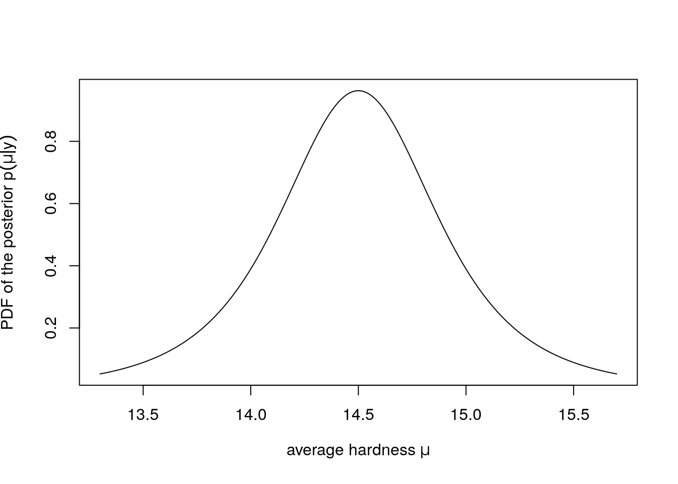
2.1 Marginal and probabilities for \(\mu\)
Write your answers and code here!
Keep the below name and format for the functions to work with markmyassignment:
# Useful functions: mean(), length(), sqrt(), sum()
# and qtnew(), dtnew() (from aaltobda)

mu_point_est <- function(data) {
    # Do computation here, and return as below.
    # This is the correct return value for the test data provided above.
    14.5

}
mu_interval <- function(data, prob = 0.95) {
    # Do computation here, and return as below.
    # This is the correct return value for the test data provided above.
    c(13.3, 15.7)

}
You can plot the density as below if you implement mu_pdf to compute the PDF of the posterior \(p(\mu|y)\) of the average hardness \(\mu\).
mu_pdf <- function(data, x){
    # Compute necessary parameters here.
    # These are the correct parameters for `windshieldy_test`
    # with the provided uninformative prior.
    df = 3
    location = 14.5
    scale = 0.3817557
    # Use the computed parameters as below to compute the PDF:

    dtnew(x, df, location, scale)
}

x_interval = mu_interval(windshieldy1, .999)
lower_x = x_interval[1]
upper_x = x_interval[2]
x = seq(lower_x, upper_x, length.out=1000)
plot(
    x, mu_pdf(windshieldy1, x), type="l",
    xlab=TeX(r'(average hardness $\mu$)'),
    ylab=TeX(r'(PDF of the posterior $p(\mu|y)$)')
)
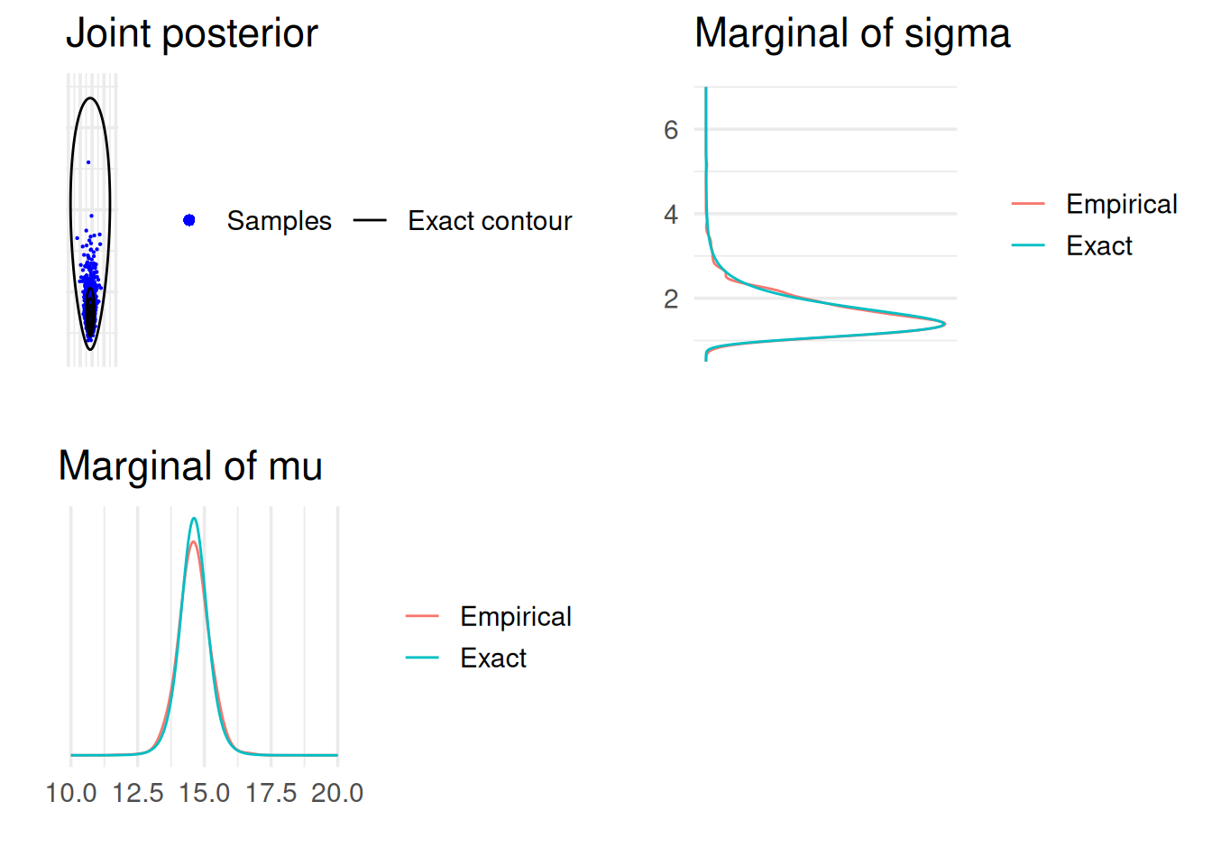
2.2 Joint posterior distribution for \(\mu\) and \(\sigma\)
# Define the inputs for the below: Sufficient Statistics
y <- windshieldy1
n <- length(y)
s2 <- var(y)
my <- mean(y)

# helper functions to sample from and evaluate
# scaled inverse chi-squared distribution
rsinvchisq <- function(n, nu, s2, ...) nu*s2 / rchisq(n , nu, ...)
dsinvchisq <- function(x, nu, s2){
  exp(log(nu/2)*nu/2 - lgamma(nu/2) + log(s2)/2*nu - log(x)*(nu/2+1) - (nu*s2/2)/x)
}


# Sample 1000 draws from marginal posteriors
ns <- 1000
sigma2  <- rsinvchisq(ns, n-1, s2)
mu <- my + sqrt(sigma2/n)*rnorm(length(sigma2))
sigma <- sqrt(sigma2)

# Compute the density in a grid of ranged for the grids
t1l <- c(10, 20)
t2l <- c(0.5, 7)
nl <- c(0.001, 50)
t1 <- seq(t1l[1], t1l[2], length.out = ns)
t2 <- seq(t2l[1], t2l[2], length.out = ns)


# Compute the exact marginal density of mu:
# multiplication by 1./sqrt(s2/n) is due to the transformation of
# variable z=(x-mean(y))/sqrt(s2/n), see BDA3 p. 21
pm <- dt((t1-my) / sqrt(s2/n), n-1) / sqrt(s2/n)

# Estimate the marginal density using samples and ad hoc Gaussian kernel approximation
pmk <- density(mu, adjust = 2, n = ns, from = t1l[1], to = t1l[2])$y

#Compute the exact marginal density of sigma:
# the multiplication by 2*t2 is due to the transformation of
# variable z=t2^2, see BDA3 p. 21
ps <- dsinvchisq(t2^2, n-1, s2) * 2*t2

# Estimate the marginal density using samples and ad hoc Gaussian kernel approximation
psk <- density(sigma, n = ns, from = t2l[1], to = t2l[2])$y


# Evaluate the joint density in a grid. Note that the following is not normalized, but for plotting contours it does not matter :
# Combine grid points into another data frame
# with all pairwise combinations
dfj <- data.frame(t1 = rep(t1, each = length(t2)),
                  t2 = rep(t2, length(t1)))
dfj$z <- dsinvchisq(dfj$t2^2, n-1, s2) * 2*dfj$t2 * dnorm(dfj$t1, my, dfj$t2/sqrt(n))
# breaks for plotting the contours
cl <- seq(1e-5, max(dfj$z), length.out = 6)


# Now, visualise the joint and marginal densities
dfm <- data.frame(t1, Exact = pm, Empirical = pmk) |>
  pivot_longer(cols = !t1, names_to="grp", values_to="p")
margmu <- ggplot(dfm) +
  geom_line(aes(t1, p, color = grp)) +
  coord_cartesian(xlim = t1l) +
  labs(title = 'Marginal of mu', x = '', y = '') +
  scale_y_continuous(breaks = NULL) +
  theme(legend.background = element_blank(),
        legend.position.inside = c(0.75, 0.8),
        legend.title = element_blank())


dfs <- data.frame(t2, Exact = ps, Empirical = psk) |>
  pivot_longer(cols = !t2, names_to="grp", values_to="p")
margsig <- ggplot(dfs) +
  geom_line(aes(t2, p, color = grp)) +
  coord_cartesian(xlim = t2l) +
  coord_flip() +
  labs(title = 'Marginal of sigma', x = '', y = '') +
  scale_y_continuous(breaks = NULL) +
  theme(legend.background = element_blank(),
        legend.position.inside = c(0.75, 0.8),
        legend.title = element_blank())
Coordinate system already present.
ℹ Adding new coordinate system, which will replace the existing one.joint1labs <- c('Samples','Exact contour')
joint1 <- ggplot() +
geom_point(data = data.frame(mu,sigma), aes(mu, sigma, col = '1'), size = 0.1) +
geom_contour(data = dfj, aes(t1, t2, z = z, col = '2'), breaks = cl) +
coord_cartesian(xlim = t1l,ylim = t2l) +
labs(title = 'Joint posterior', x = '', y = '') +
scale_y_continuous(labels = NULL) +
scale_x_continuous(labels = NULL) +
scale_color_manual(values=c('blue', 'black'), labels = joint1labs) +
guides(color = guide_legend(nrow = 1, override.aes = list(
shape = c(16, NA), linetype = c(0, 1), size = c(2, 1)))) +
theme(legend.background = element_blank(),
legend.position.inside = c(0.5, 0.9),
legend.title = element_blank())
# blank plot for combining the plots
bp <- grid.rect(gp = gpar(col = 'white'))
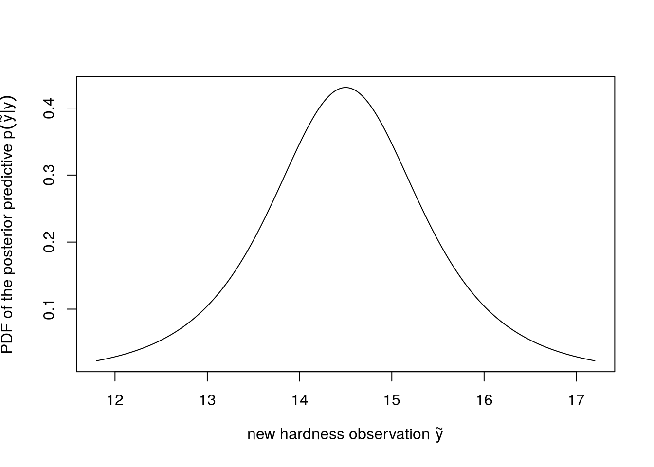
2.3 Predictive distribution
Write your answers and code here!
Keep the below name and format for the functions to work with markmyassignment:
# Useful functions: mean(), length(), sqrt(), sum()
# and qtnew(), dtnew() (from aaltobda)

mu_pred_point_est <- function(data) {
    # Do computation here, and return as below.
    # This is the correct return value for the test data provided above.
    14.5

}
mu_pred_interval <- function(data, prob = 0.95) {
    # Do computation here, and return as below.
    # This is the correct return value for the test data provided above.
    c(11.8, 17.2)

}
You can plot the density as below if you implement mu_pred_pdf to compute the PDF of the posterior predictive \(p(\tilde{y}|y)\) of a new hardness observation \(\tilde{y}\).
mu_pred_pdf <- function(data, x){
    # Compute necessary parameters here.
    # These are the correct parameters for `windshieldy_test`
    # with the provided uninformative prior.
    df = 3
    location = 14.5
    scale = 0.8536316
    # Use the computed parameters as below to compute the PDF:

    dtnew(x, df, location, scale)
}

x_interval = mu_pred_interval(windshieldy1, .999)
lower_x = x_interval[1]
upper_x = x_interval[2]
x = seq(lower_x, upper_x, length.out=1000)
plot(
    x, mu_pred_pdf(windshieldy1, x), type="l",
    xlab=TeX(r'(new hardness observation $\tilde{y}$)'),
    ylab=TeX(r'(PDF of the posterior predictive $p(\tilde{y}|y)$)')
)
3 Inference for the difference between proportions
An experiment was performed to estimate the effect of beta-blockers on mortality of cardiac patients. A group of patients was randomly assigned to treatment and control groups: out of 674 patients receiving the control, 39 died, and out of 680 receiving the treatment, 22 died. Assume that the outcomes are independent and binomially distributed, with probabilities of death of \(p_0\) and \(p_1\) under the control and treatment, respectively. Set up a noninformative or weakly informative prior distribution on \((p_0,p_1)\).
Summarize the posterior distribution for the odds ratio, \[ \mathrm{OR} = (p_1/(1-p_1))/(p_0/(1-p_0)). \]
In order to help you answering the quiz questions, we recommend you:
- Compute and report the point estimate \(E(\mathrm{OR}|y_0,y_1)\),
- compute and report a posterior 95%-interval,
- plot the histogram, and
- write interpretation of the result in text.
Use Frank Harrell’s recommendations how to state results in Bayesian two group comparison.
With a conjugate prior, a closed-form posterior is the Beta form for each group separately (see equations in the book). You can use rbeta() to sample from the posterior distributions of \(p_0\) and \(p_1\), and use this sample and odds ratio equation to get a sample from the distribution of the odds ratio.
Write your answers and code here!
The below data is only for the tests:
Keep the below name and format for the functions to work with markmyassignment:
# Useful function: mean(), quantile()
posterior_odds_ratio_point_est <- function(p0, p1) {
# Do computation here, and return as below.
# This is the correct return value for the test data provided above.
2.650172
}
posterior_odds_ratio_interval <- function(p0, p1, prob = 0.95) {
# Do computation here, and return as below.
# This is the correct return value for the test data provided above.
c(0.6796942,7.3015964)
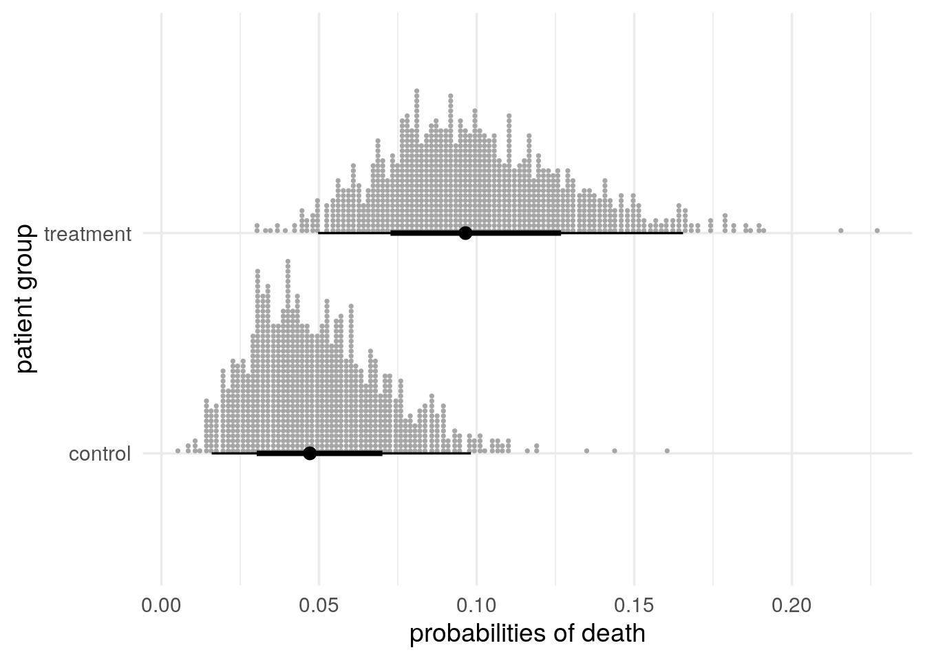
}3.1 advanced tools (posterior’s rvar, ggdist’s stat_dotsinterval)
The posterior package’s random variable datatype rvar is a “sample-based representation of random variables” which makes handling of random samples (of draws) such as the ones contained in the above variables p0 and p1 easier. By default, it prints as the mean and standard deviation of the draws, such that rvar(p0) prints as 0.05 ± 0.021 and rvar(p1) prints as 0.1 ± 0.029.
The datatype is “designed to […] be able to be used inside data.frame()s and tibble()s, and to be used with distribution visualizations in the ggdist package.” The code below sets up an R data.frame() with the draws in p0 and p1 wrapped in an rvar, and uses that data frame to visualize the draws using ggdist, an R package building on ggplot2 and “designed for both frequentist and Bayesian uncertainty visualization”.
The below plot, Figure 3 uses ggdist’s stat_dotsinterval(), which by default visualizes
- an
rvar’s median and central 66% and 95% intervals using a black dot and lines of varying thicknesses as when usingggdist’sstat_pointinterval()and - an
rvar’s draws using grey dots as when usingggdist’sstat_dots():
rvars make it easy to compute functions of random variables, such as
- differences, e.g. \(p_0 - p_1\):
r0 - r1computes anrvarwhich prints as -0.05 ± 0.037, indicating the sample mean and the sample standard deviation of the difference of the probabilities of death, - products, e.g. \(p_0 \, p_1\):
r0 * r1computes anrvarwhich prints as 0.005 ± 0.0026 which in this case has no great interpretation
Below, in Figure 4, we compute the odds ratios using the rvars and visualize its median, central intervals and draws, as above in Figure 3:
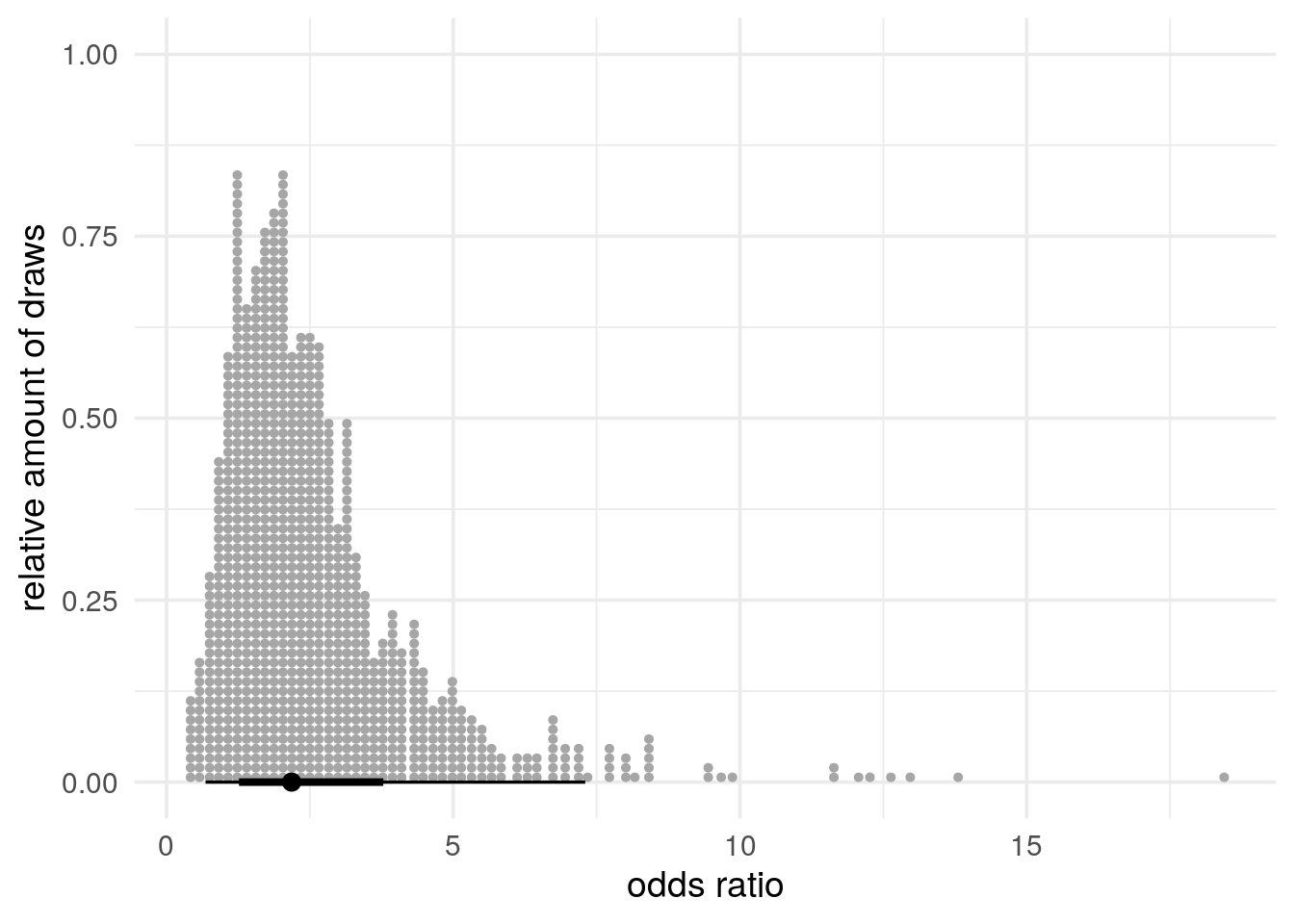
You can use Figure 4 to visually check whether the answers you computed make sense.
4 Inference for the difference between normal means
Consider a case where the same factory has two production lines for manufacturing car windshields. Independent samples from the two production lines were tested for hardness. The hardness measurements for the two samples \(\mathbf{y}_1\) and \(\mathbf{y}_2\) be found in the datasets windshieldy1 and windshieldy2 in the aaltobda package.
We assume that the samples have unknown standard deviations \(\sigma_1\) and \(\sigma_2\). Use the uninformative prior.
[1] 15.980 14.206 16.011 17.250 15.993 15.722With a conjugate prior, a closed-form posterior is Student’s \(t\) form for each group separately (see equations in the book). You can use the rtnew() function to sample from the posterior distributions of \(\mu_1\) and \(\mu_2\), and use this sample to get a sample from the distribution of the difference \(\mu_d = \mu_1 - \mu_2\).
Write your answers and code here!