Assignment 7
1 General information
The exercises here refer to the lecture 7/BDA chapter 5 content. The main topics for this assignment are the MCSE and importance sampling.
The exercises constitute 96% of the Quiz 7 grade.
We prepared a quarto notebook specific to this assignment to help you get started. You still need to fill in your answers on Mycourses! You can inspect this and future templates
- as a rendered html file (to access the qmd file click the “</> Code” button at the top right hand corner of the template)
- Questions below are exact copies of the text found in the MyCourses quiz and should serve as a notebook where you can store notes and code.
- We recommend opening these notebooks in the Aalto JupyterHub, see how to use R and RStudio remotely.
- For inspiration for code, have a look at the BDA R Demos and the specific Assignment code notebooks
- Recommended additional self study exercises for each chapter in BDA3 are listed in the course web page. These will help to gain deeper understanding of the topic.
- Common questions and answers regarding installation and technical problems can be found in Frequently Asked Questions (FAQ).
- Deadlines for all assignments can be found on the course web page and in MyCourses.
- You are allowed to discuss assignments with your friends, but it is not allowed to copy solutions directly from other students or from internet.
- Do not share your answers publicly.
- Do not copy answers from the internet or from previous years. We compare the answers to the answers from previous years and to the answers from other students this year.
- Use of AI is allowed on the course, but the most of the work needs to by the student, and you need to report whether you used AI and in which way you used them (See points 5 and 6 in Aalto guidelines for use of AI in teaching).
- All suspected plagiarism will be reported and investigated. See more about the Aalto University Code of Academic Integrity and Handling Violations Thereof.
- If you have any suggestions or improvements to the course material, please post in the course chat feedback channel, create an issue, or submit a pull request to the public repository!
- The decimal separator throughout the whole course is a dot, “.” (Follows English language convention). Please be aware that MyCourses will not accept numerical value answers with “,” as a decimal separator
- Unless stated otherwise: if the question instructions ask for reporting of numerical values in terms of the ith decimal digit, round to the ith decimal digit. For example, 0.0075 for two decimal digits should be reported as 0.01. More on this in Assignment 4.
1.1 Assignment questions
For convenience the assignment questions are copied below. Answer the questions in MyCourses.
Lecture 7/Chapter 5 of BDA Quiz (96% of grade)
This week’s assignment focuses on hierarchical models and modelling with brms.
1. Exchangeability
An important building block of hierarchical models is the assumption of exchangeability. Please have a look at lecture 7, slides 75-83, Chapter 5.2 in BDA3, as well as the chapter notes for chapter 5 more details on the difference between the exchangeability and independence assumption. Let’s review.
1.1 Consider parameters \(\theta_j\) for \(j \; \text{in} \; 1...J\). Which of these statements correctly describes exchangeability?
1.2 What best describes the difference between independence and exchangeability?
Consider the following: assume a box has n black and white balls but we do not know how many of each color. We pick a ball \(y_1\) at random, we do not put it back, and pick another ball \(y_2\) at random. Denote the number of black balls by B and white by W.
1.3 Are observations \(y_1\) and \(y_2\) exchangeable?
1.4 Are observations \(y_1\) and \(y_2\) independent?
1.5 Can we treat the two observations as if they are independent?
1.6 Exchangeability allows us to express dependencies of data and parameters in a convenient form. Suppose we model a sequence of exchangeable random variables \(\theta\) via a governing, or population distribution, where conditional on some unknown parameters \(\phi\), we may assume independence between the elements of \(\theta\). Assume that \(\theta\) has \(J\) elements, write down an equation that conveniently factors the joint probability \(p(\theta,\phi)\):
De Finetti’s theorem provides the theoretical basis for the equivalence to the independence assumption when \(J\) goes to infinity. In practice \(J\) is finite, but the difference may be small when \(J\) is relatively large. Check out the examples mentioned in the Chapter notes if you need more convincing.
\(\phi\) is in general unknown. So the marginal prior for \(\theta\) must average over uncertainty in \(\phi\): \(\int \prod_{j=1}^Jp(\theta_j \mid \phi)p(\phi)d\phi\).
1.7 Based on the marginal prior formulation in the paragraph above, what can you say about the covariances \(\mathrm{cov}(\theta_i,\theta_j)\)?
1.8 As with the parameters above, we often think of exchangeability as arising for our data model conditional on extra information \(x\), such that the tuple \((x_i,y_i)\) are exchangeable whereas \(y_i\) might not be. In which modeling context is this useful? Assume that the target data is denoted by \(y_i\).
2. Overview of hierarchical models
2.1 Which of these best describes a hierarchical model?
2.2 Consider that there are observations \(y\) indexed by observation number \(i\) and group \(j\). Suppose the data are modeled dependent on parameters \(θ_j\) where \(j=1,\dotsc,J\) indexes some meaningful grouping such as hospital-j specific health-outcomes, conditional on parameters \(\phi\) which are hyper-parameters of the prior distribution of \(\theta_j\). \(\phi\) are modeled by prior distribution \(p(\phi)\). We think of the distribution \(p(\theta_j|\phi)\) as the population distribution which generates the values for \(\theta\) in the hierarchical model. What are some of the benefits of hierarchical models compared to separate models, which assume no relationship between \(j\) (and separate models are estimated), and pooled models, which consider all \(j\) jointly, but do not model \(j\) specific parameters?
Throughout the rest of the course, we will often compare the hierarchical model, to a separate model and the pooled model. Suppose for the questions below that you are modeling data \(y_{ij}\) where \(i\) refers to an observation within the jth group, the observation model for \(y_{ij}\) is normal, and we consider hierarchies at the level of the parameters describing the location of \(y_{ij}\).
2.3 Based on the description of the above, the lecture and BDA chapter 5 content, which of these below would suggest a separate model for \(y_{ij}\)? \(\pi()\) stands for some prior distribution and \(η_j\) may be a vector of parameters such that \(\mathrm{cov}(\eta_s,\eta_r)=0\) for \(s\neq r\).
2.4 Based on the description of the above, the lecture and BDA chapter 5 content, which of these below would suggest a pooled model for \(y_{ij}\)? \(\pi()\) stands for some prior distribution and \(η_j\) may be a vector of parameters such that \(\mathrm{cov}(\eta_s,\eta_r)=0\) for \(s\neq r\).
2.5 Based on the description of the above, the lecture and BDA chapter 5 content, which of these below would suggest a hierarchical model for \(y_{ij}\)? \(\pi()\) stands for some prior distribution and \(η_j\) may be a vector of parameters such that \(\mathrm{cov}(\eta_s,\eta_r)=0\) for \(s\neq r\).
2.6 Why are hierarchical models sometimes also referred to as partially pooled models. You may find it helpful to review the first unnumbered equation on page 115 of BDA3?
It may help, before translating the model to code, to first describe the relationship between variables as a directed acyclic graph (DAG) (see lecture 7,slide 3). We interpret the DAG starting from top to bottom as describing the generative mechanism implied by priors and observation model for \(y_{ij}\). Top level variables feed into distributions of lower level parameters and the observation model. Distributions are typically not further described in the DAG. By drawing variables sequentially from top to bottom, you can generate fake observations (push-forward distribution). In the case that the parameters have not yet been updated by the data information, this push-forward distribution is called the prior predictive distribution of \(y\). You have already created such a prior predictive distribution in Assignment 1, question 7 and we will return to this in the sections below.
2.7 What is the difference between sequential draws from priors and the data model as described above to drawing from the joint posterior in Stan?
In the Figure 1 below, assume that all circular nodes indicate that the object inside can be generated according to some distribution, conditional on the parent nodes.
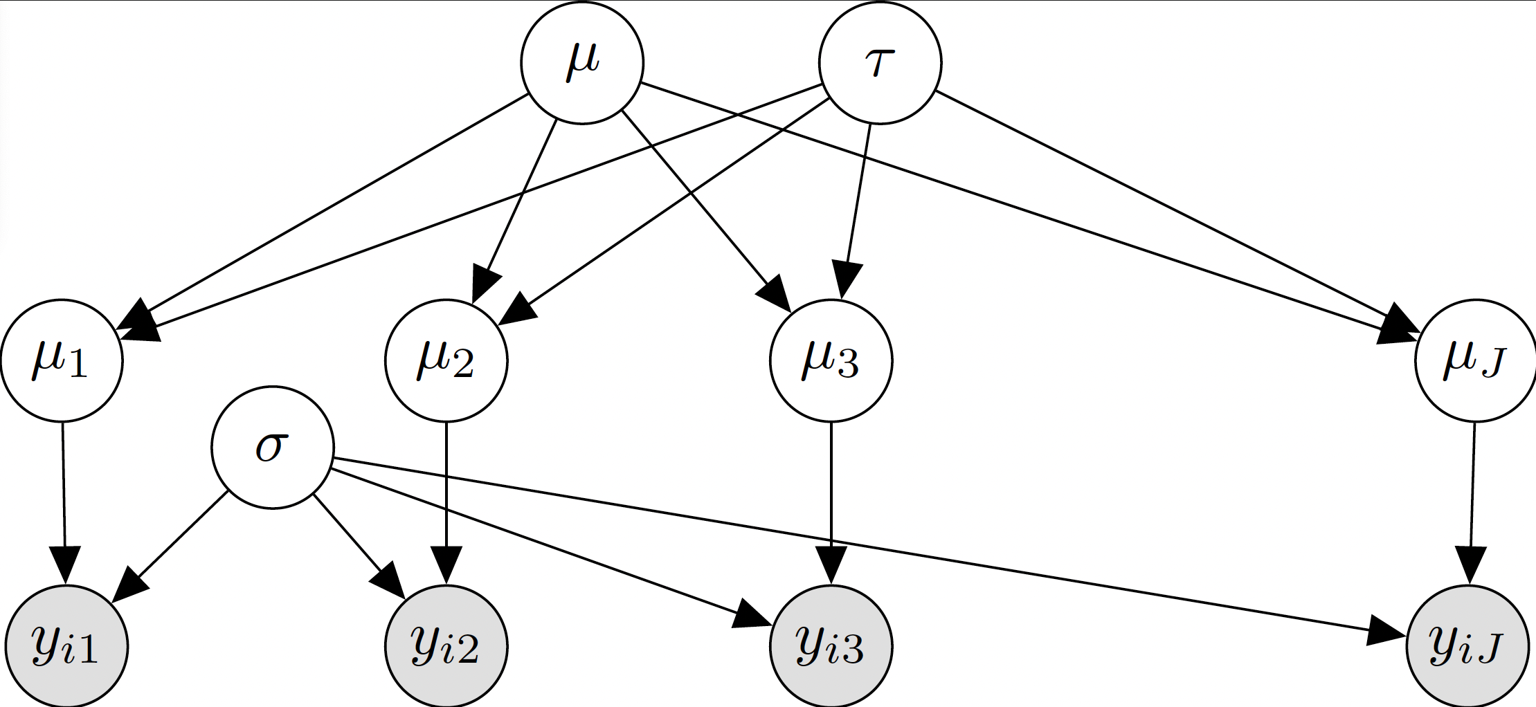
Figure 1
2.8 Which of these equations properly describes the posterior for the model shown in the diagram?
3. Meta-analysis and hierarchical models
Often similar research studies in areas such as medicine or social science will be published under slightly different conditions or replicated with different subjects. It is of interest to summarise and integrate those findings for which hierarchical models have become increasingly popular.
3.1 Suppose \(y_i\) is the point estimate for an effect size of a single study, \(i\). Why is it often appropriate to model \(y_i\) by a normal distribution with known standard deviation \(\sigma_i\) which is taken as the standard error estimate for \(y_i\)?
3.2 Why are hierarchical models preferable to separate and pooled models for meta-analysis?
3.3 Suppose the assumption of exchangeability is false because you know the estimates of effects across studies depends on extra information \(x_i\), e.g. geolocation, and this has a substantial impact on the estimates. What should you do in this circumstance?
3.4 Based on the discussion above, which of the below would refer to a hierarchical model for \(y_i\)?
4. Introduction to brms
brms is an R package which makes writing models with Stan easier.
Suppose you have oberved the following variables, from different groups: \(x,z,y\). \(i\) is the observation number and \(j\) the group indicator. Assume a model \(y_{ij} \sim \mathrm{normal}\left(\mu_{ij},\sigma\right)\). Translate the following equations for the linear predictor term \(\mu_{ij}\) into brms syntax:
4.1 \(\mu_{ij}=\alpha_0\):
4.2 \(\mu_{ij}=\alpha_0+\beta_1 x_i\)
4.3 \(\mu_{ij}=\alpha_0+\beta_1 x_i+\beta_2 z_i\)
4.4 \(\mu_{ij}=\alpha_0+\alpha_j+\beta_1 x_i\)
Note that in within brms, coefficients that do not vary according to some grouping index (e.g. \(\mu_{ij}=\alpha_0\)) are called population effects while coefficients that vary according to some grouping are called varying effects (e.g. \(\mu_{ij}=\alpha_j\)). Some literatures refer to these parameters as fixed and random effects respectively, however in the context of Bayesian inference, this terminology can be misleading, since parameters in a model are treated as random variables. See here for more discussion on this. For the questions below, we will use brms terminology.
5. Simulation warmup
In this task, you will simulate data from a hierarchical model to gain better insight into it.
The following R code simulates data from a hierarchical structure, and then plots the results. Experiment with this function by using it on different values of the arguments, and answer the following questions. This code is also included in the notebook for this assignment.
hierarchical_sim <- function(group_pop_mean,
                             between_group_sd,
                             within_group_sd,
                             n_groups,
                             n_obs_per_group
                             ) {
  # Generate group means
  group_means <- rnorm(n = n_groups, mean = group_pop_mean, sd = between_group_sd)
  # Generate observations
  ## Create an empty vector for observations
  y <- numeric()
  ## Create a vector for the group identifier
  group <- rep(1:n_groups, each = n_obs_per_group)
  for (j in 1:n_groups) {
    ### Generate one group observations
    group_y <- rnorm(n = n_obs_per_group, mean = group_means[j], sd = within_group_sd)
    ### Append the group observations to the vector
    y <- c(y, group_y)
  }
  # Combine into a data frame
  data <- data.frame(group = factor(group), y = y)
  # Plot the data
  ggplot(data, aes(x = y, y = group)) +
    geom_point() +
    geom_vline(xintercept = group_pop_mean, linetype = "dashed")
}
5.1 Which of the following generative models does the code correspond to? \(i\) is the observation number, \(j\) is the group indicator.
5.2 What does the vertical dashed line in the plot represent?
5.3 Which function call would plausibly create Figure 2 below (although the random numbers you generate will almost certainly be different those plotted below, try to distill what attributes are captured with the different simulation choices and compare to the below)?
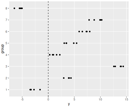
Figure 2
5.4 Which of these statements correctly describes the behaviour when the number of groups is increased?
5.5 Which of these statements correctly describes the behaviour when the ratio of the between group and within group variance is changed?
6. Sleep deprivation
In many studies, data will have been collected for the same people repeatedly (e.g. at different time points). A hierarchical model is well suited for such data as we can specify a grouping structure corresponding to the person/subject id. The sleepstudy dataset contains observations of reaction times for different people after differing number of days of sleep deprivation.
Your task is to fit a hierarchical normal linear model in brms. The observation model will be \(\mathrm{Reaction}_{ij} \sim \mathrm{normal}\left(\mu_{ij},\sigma\right)\) where \(i\) refers to an observation id and \(j\) to the subject id. But depending on the model, the \(\mu_{ij}\) term will be differently parameterised.
First fit a model with a population-level intercept, population-level effect
of Days and varying intercept per Subject. Note: in order to have the
Intercept parameter be more clearly interpretable, use center =
FALSE when creating the brms formula (see the Parameterization of the
population-level intercept secion in the brms manual.
Centering refers here to data transformations made within the Stan model, that
among other things makes sampling more efficient, but change the
interpretation of the intercept. Section
5 of this demo provides some more insight into this. Use the following
priors (check the code notebook for how to specify):
\(\alpha_0 \sim \mathrm{normal}\left(250,100\right); \beta_0 \sim \mathrm{normal}\left(0,20\right);\alpha_j \sim \mathrm{normal}\left(0,\tau\right); \tau \sim \mathrm{normal}_+\left(0,100\right);\sigma \sim \mathrm{normal}_+\left(0,100\right)\)
6.1 Which of these formulae correctly defines the linear predictor term in a model with population-level intercept, population-level effect of Days and varying intercepts per Subject?
6.2 Which is the correct brms formula for this model?
6.3 Based on the posterior, the estimate of the population-level intercept is:
6.4 The population-level intercept can be interpreted as:
6.5 Based on the posterior, the estimate of the population-level effect of Days on Reaction \(i\):
6.6 The population-level effect of Days can be interpreted as:
6.7 Based on the posterior, the estimate of the standard deviation of the Intercept between Subjects \(i\):
6.8 The standard deviation of the Subject-specific Intercept can be interpreted as:
Next fit a model with Subject-specific effects of Days in addition to the other terms.
In this model, we can consider a correlation between the by-Subject Intercept and Days effects. This means the priors on \(\alpha_j\) and \(\beta_j\) can be considered as a multivariate normal \(\left(\alpha_j,\beta_j\right)\sim \mathrm{N}\left(0,\Sigma\right)\). It is common to decompose this into a prior on \(\alpha_j\) and \(\beta_j\) and a prior on the correlation matrix \(R\).
Use the priors \(\alpha_j \sim \mathrm{normal}\left(0,\tau_\alpha\right), \beta_j\sim \mathrm{normal}\left(0,\tau_\beta\right), \tau_\alpha\sim \mathrm{normal}_+\left(0,100\right), \tau_\beta\sim \mathrm{normal}_+\left(0,20\right)\) and \(R\sim \mathrm{LKJ}\left(2\right)\).
6.9 Which of these formulae correctly defines the linear predictor in this case?
6.10 Which is the correct brms formula for this model?
6.11 Based on the posterior, the estimate of the standard deviation of Subject-specific effect of Days is:
6.12 Based on the posterior, the estimate of correlation between the Subject-specific Intercept and effect of Days is:
6.13 After fitting both models, which of the statements describe the results best (here interpret “plausible” as what is contained within the 95% posterior interval):
Based on this, we would hope to see also graphically differences between the
varying intercept only and the varying intercept plus varying slope models.
Use the conditional_effect() function in brms to plot the
posterior distribution of the linear predictor term at the covariate’s mean
values (this
is the default of the function).
First, let’s check you used the function correctly.
6.14 Which figure plots the conditional effects of the varying slope model?
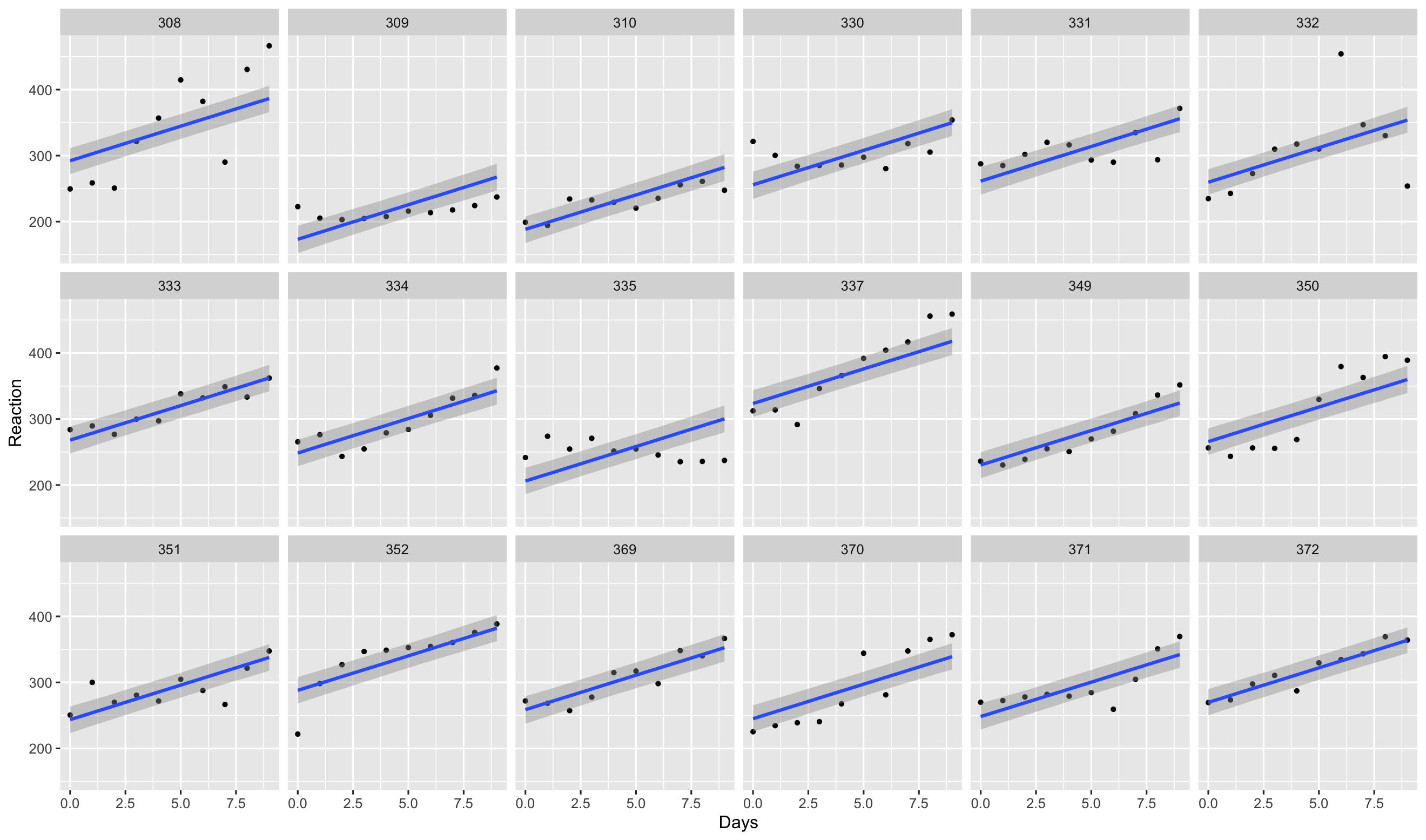
Figure 3
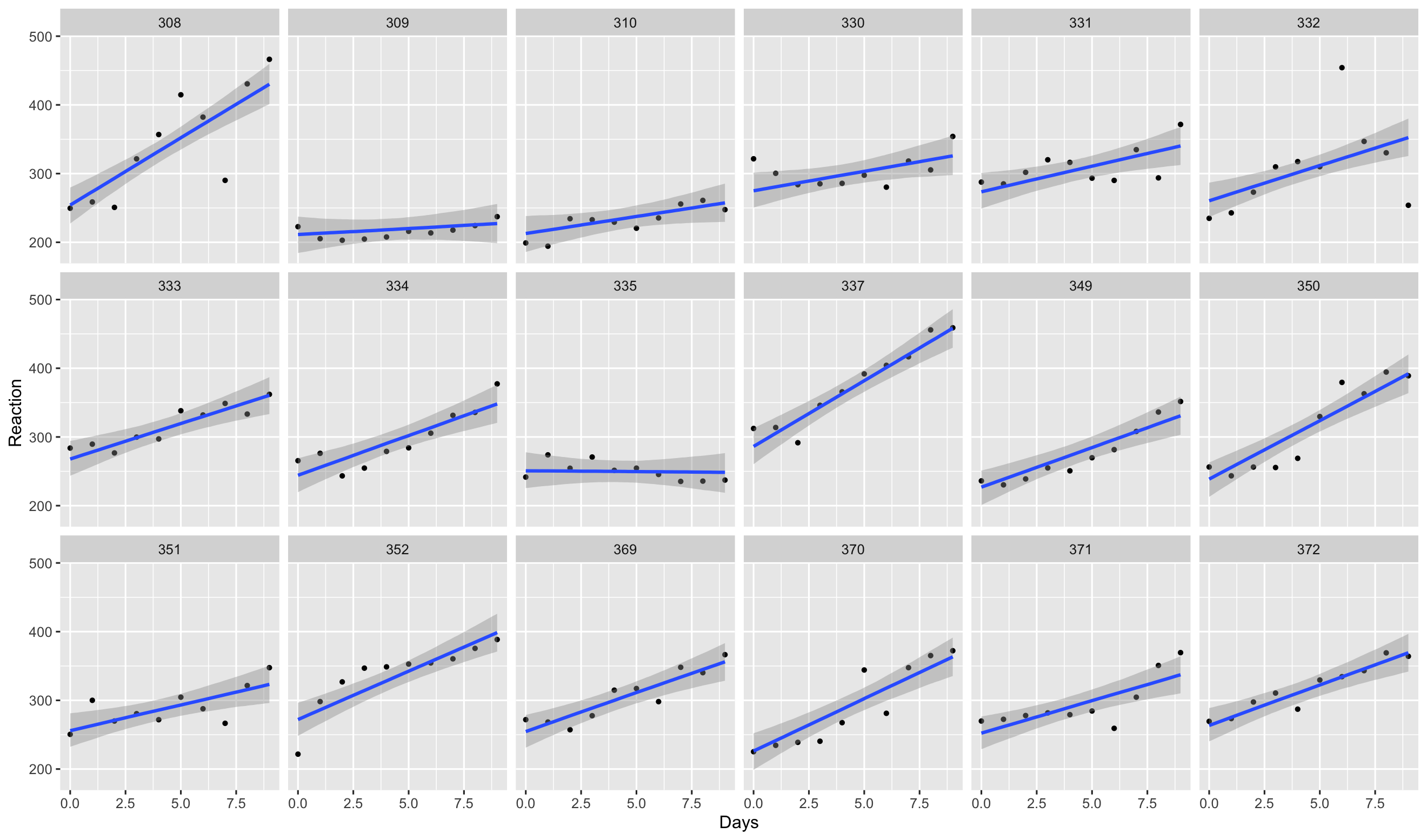
Figure 4
We will add more model features and conduct predictive evaluation in the next assignment!
7. School calendar dataset
As you’ve learned from the above, hierarchical models are also useful for meta-analyses.
The dataset dat.konstantopolous2011 from the
metadat package contains results from different studies conducted
on the effect of changing the school calendar from a standard one with a long
summer break to a modified one with more regular but shorter breaks.
Each result of a study is a standardized estimated mean effect on student achievement, where positive values indicate improvement \((y_i)\) and the variance of the estimate \((v_i)\) for a school.
The meta-analysis model can be written as follows: \(y_{ijk} \sim \mathrm{normal}\left(\mu_{ijk},\sigma_{ijk}\right)\). \(i\) refers to an observation, \(j\) refers to a school, \(k\) refers to a district. \(\mu_{ijk}\) thus refers to one observation \(i\) at school \(j\) in district \(k\). \(\mu_0\) is the population-level effect, \(\mu_j\) is the school-specific effect, and \(\mu_k\) is the district-specific effect.
In this case, the \(\sigma_{ijk}\) values are known (the standard errors reported from each study) and the \(\mu_{ijk}\) term will differ depending on the model.
In this exercise you will fit four different models to the same data set: Pooled, separate, partially pooled within school-specific effects, and partially pooled within schools and district effects.
For all models, use brms with the default priors and use the following settings: iter = 2000, warmup = 1000, chains = 4, seed = 2024
The dataset has separate columns for school and district, but for the models, we will want a unique identifier for each school. Before fitting any models, add a new column to the dataset called “district_school” which is the combination of the district and the school. This is then unique for each school, and will be used in the model formulae.
Pooled model:
Use brms to fit a pooled model and answer the following questions. Check the code notebook for help starting.
The pooled model formula is: \(\mu_{ijk}=\mu_0\).
7.1 The pooled model is written as:
7.2 How many parameters are estimated in the pooled model?
7.6 Based on the posterior of the Intercept, what would you conclude about the effect of the intervention:
7.7 Suppose there is a new school in an existing district
(School = 9, District = 86). What is the mean prediction for the effect in
this school? Use the function posterior_epred and the newdata
argument.
Use brms to fit a separate model and answer the following questions. Check the code notebook for help starting.
The separate model formula is: \(\mu_{ijk}=\mu_{jk}\).
7.9 The separate model is written as:
7.10 How many parameters are estimated in the separate model?
Mean: , lower 95% interval bound: , upper 95% interval bound:
7.12 What is the estimated effect for School 7 in District 86?
Mean: , lower 95% interval bound: , upper 95% interval bound:
7.13 Based on the posterior for the separate model, what could reasonably be concluded about the effect of the intervention:
7.14 Suppose there is a new school in an existing district (District = 86, School = 9). Why can we not easily predict the effect for this school based on the separate model posterior?
Partially pooled model for schools
The partially pooled model formula is: \(\mu_{ijk} = \mu_0 + \mu_{jk}\)
7.15 And the partially pooled hierarchical model:
7.16 How many parameters are estimated in the partially pooled for schools model?
7.18 What is the estimated effect for School 3 in District 71?
Mean: , lower 95% interval bound: , upper 95% interval bound:
7.19 What is the estimated effect of School 7 in District 86?
Mean: , lower 95% interval bound: , upper 95% interval bound:
7.20 Suppose there is a new school in an existing district
(District = 86, School = 9). What would the mean prediction for the effect in
this school? Use the functionposterior_epred and the newdata
argument with allow_new_levels = TRUE:
In this data set, as there is a two-level structure, where schools are nested in districts, we can add another level to the hierarchy. The additional hierarchy formula is: \(\mu_{ijk}=\mu_0+\mu_j+\mu_{jk}\)
7.22 What is the correct brms formula?
7.23 How many parameters are estimated in the partially pooled for schools in districts model?
7.27 After fitting all the models, choose which of the following statements relating to the results are true: