Assignment 5
1 General information
The exercises here refer to the lecture 5/BDA chapter 11 content. The main topics for this assignment are the MCSE and importance sampling.
The exercises constitute 96% of the Quiz 5 grade.
We prepared a quarto notebook specific to this assignment to help you get started. You still need to fill in your answers on Mycourses! You can inspect this and future templates
- as a rendered html file (to access the qmd file click the “</> Code” button at the top right hand corner of the template)
- Questions below are exact copies of the text found in the MyCourses quiz and should serve as a notebook where you can store notes and code.
- We recommend opening these notebooks in the Aalto JupyterHub, see how to use R and RStudio remotely.
- For inspiration for code, have a look at the BDA R Demos and the specific Assignment code notebooks
- Recommended additional self study exercises for each chapter in BDA3 are listed in the course web page. These will help to gain deeper understanding of the topic.
- Common questions and answers regarding installation and technical problems can be found in Frequently Asked Questions (FAQ).
- Deadlines for all assignments can be found on the course web page and in MyCourses.
- You are allowed to discuss assignments with your friends, but it is not allowed to copy solutions directly from other students or from internet.
- Do not share your answers publicly.
- Do not copy answers from the internet or from previous years. We compare the answers to the answers from previous years and to the answers from other students this year.
- Use of AI is allowed on the course, but the most of the work needs to by the student, and you need to report whether you used AI and in which way you used them (See points 5 and 6 in Aalto guidelines for use of AI in teaching).
- All suspected plagiarism will be reported and investigated. See more about the Aalto University Code of Academic Integrity and Handling Violations Thereof.
- If you have any suggestions or improvements to the course material, please post in the course chat feedback channel, create an issue, or submit a pull request to the public repository!
- The decimal separator throughout the whole course is a dot, “.” (Follows English language convention). Please be aware that MyCourses will not accept numerical value answers with “,” as a decimal separator
- Unless stated otherwise: if the question instructions ask for reporting of numerical values in terms of the ith decimal digit, round to the ith decimal digit. For example, 0.0075 for two decimal digits should be reported as 0.01. More on this in Assignment 4.
1.1 Assignment questions
For convenience the assignment questions are copied below. Answer the questions in MyCourses.
Lecture 5/Chapter 11 of BDA Quiz (96% of grade)
1. Monte Carlo Methods
As you’ve learned in the previous assignments, in some cases we have closed form solution for useful posterior summaries for parameter vector \(\theta\).
1.1 Why are Monte Carlo and other sampling based methods for posterior evaluation of functions \(f(\theta)\) convenient?
We now briefly review some Monte Carlo methods. Assume we want to obtain draws from \(p(\theta \mid y)\) . Possibly the simplest way, is to apply grid sampling (see lectures 3.2 and 4.1). Briefly, the general idea of this method is to identify range of values for \(\theta\) which captures almost all the mass of the posterior distribution, divide this range into grid (small intervals for 1D case, small squares for 2D case and so on), compute the unnormalised posterior density at a grid of values, normalize them by approximating the distribution as a step function over the grid and setting the total probability in the grid to 1. Then we can draw from the discrete distribution over values of a grid (more information can be found on page 76 of BDA3). However, this approach poses a certain challenge for the case of multivariate \(\theta\).
1.2 What is the main issue of grid sampling:
We may try to apply more elaborated methods such as rejection sampling (page 264 of BDA3). Rejection sampling is based on defining a positive function \(g(\theta)\), so that we can obtain draws from the probability density proportional to \(p(\theta)\) and accept those draws according to a certain rule (check lecture 4).
1.3 What problem(s) appear with rejection sampling:
2. Markov Chain Monte Carlo (MCMC)
The most popular way to obtain posterior draws nowadays is MCMC.
2.1 What is a Markov chain?
2.2 Which of the following is not a Markov chain?
2.3 In question 2.2 we assumed discrete sequences. For the continuous case, we can use conditional transition distribution \(T_t(\theta^t \theta^{t-1})\) for a set of random variables \(\theta_1, \theta_2, \dots\) to describe the probability density \(p(\theta^t \mid \theta^1, \dots, \theta^{t-1}) = p(\theta^t \theta^{t-1})\), given some initial point \(\theta^0\). What are the two steps we need to prove for the Markov chain to eventually produce valid series of draws from the posterior \(p(\theta \mid y)\)?
2.4 What are the necessary and sufficient conditions to prove that a Markov chain has a unique stationary distribution?
2.5 Why is it often necessary to discard the first draws of the MCMC chain?
2.6 Why might MCMC be preferable to grid and rejection sampling?
3. Metropolis algorithm
The Metropolis algorithm is a relatively simple MCMC algorithm, yet it is foundational for more advanced algorithms, such as the Hamiltonian Monte Carlo algorithm you will encounter later in the course. Later in this assignment, you will implement the Metropolis algorithm (page 278 of BDA3). Denote the proposal distribution at time \(t\) for parameter vector \(\theta^t\) conditional on \(\theta^{t-1}\) as \(J_t(\theta^t \mid \theta^{t-1})\). For simplicity, we consider here symmetric proposal distributions (otherwise the algorithm would be known as the Metropolis-Hastings algorithm).
3.1 What is a main idea behind the Metropolis algorithm?
3.2: Denote the current proposal by \(\theta^*\) at time \(t\) from the proposal distribution \(J_t (\theta^* \theta^{t-1})\). Which one is the correct acceptance ratio, \(r\):
3.3 Which one is the correct rule for accepting the proposal? Denote the acceptance ratio you’ve determined in 3.2 by \(r\). Set \(\theta^t\) equal to:
3.4 Assume the posterior surface has a unique mode. What would eventually happen to the MCMC chain if adopting the rule \(\theta^*\) iff \(r > 1\) and \(\theta^{t-1}\) otherwise?
3.5 Retain the assumption made in question 3.4. Why is the posterior mode alone not generally useful for posterior expectations?
4. Trace plot diagnostics
Suppose you’ve successfully obtained multiple chains of MCMC draws from the Metropolis algorithm. Remember that the goal for the MCMC chains is to firstly converge to some unique distribution, and that all chains converge to the same distribution (with the hope of that being \(p(\theta \mid y)\)). You would now like to check if your chains can be trusted to have done so, after having discarded an appropriate amount of draws you used for warm-up. There are multiple convergence diagnostics and we will discuss some of them here. One way is to investigate the trace plot: check visually whether the chains converged to the same distribution. If they have, we say the chains have mixed. To do this, we plot them in the same figure and observe if something went wrong. Below you are given an example with two chains. Look at them carefully and answer questions below.
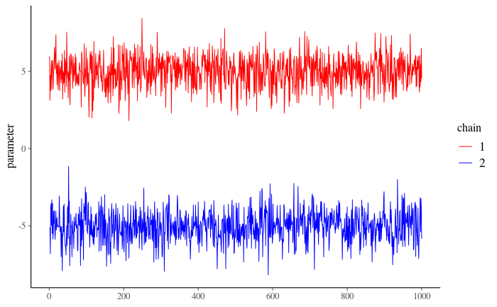
Figure 1
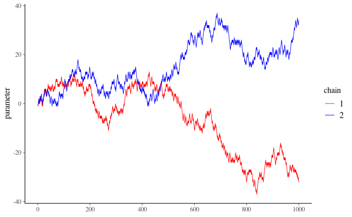
Figure 2
4.1 Can you say that your chains converged to the same distribution based on Figure 1:
4.2: Can you say that your chains are mixing well based on Figure 2:
5. Trace plot inspection can be useful when the number of parameters is small. When dealing with a large number of parameters, however, it becomes inconvenient to analyse trace plots of each parameter separately, therefore we would like to also have some quantitative metrics for investigating convergence. One of them is called Rhat. There are different versions of it, for instance, version from BDA3 book (page 285). The much improved version you will use throughout the course is presented in Vehtari et al. (2021). Let’s look at the book version to understand why it is preferred to use the modified version.
5.1: What is the definition of Rhat from the BDA3 book:
5.2: Which range of values for Rhat would are a good indicator for convergence (see lecture 5)?
Imagine a situation where one chain converged to N(0, 1) distribution and the other one to Student t with 3 degrees of freedom. The trace plot then looks like:
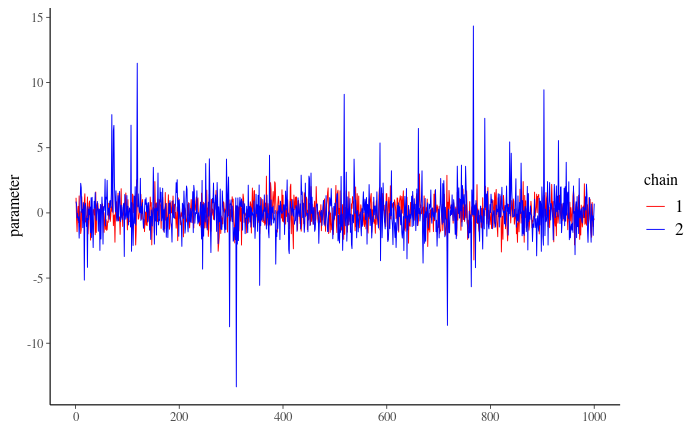
Figure 3
5.3: What do you observe?
5.4 However, despite of this issue, the Rhat value from the book equals \(\sim\) 1, indicating good convergence of the chains. What can be the explanation for this:
On the contrary, the much improved Rhat computation as presented in Vehtari et al. (2021), equals in a Rhat value of 1.39, much bigger than the recommended threshold of 1.01. You can find more examples about the usefulness of the improved Rhat computation in the paper but also this demo. The improved Rhat is the default in cmdstan as well as the brms R package (used heavily in later assignments) and is called in this assignment’s template via the posterior package.
6. ESS diagnostics
Another useful quantity is the effective sample size.
6.1: Why can we not rely on total sample size of draws from MCMC?
6.2 Suppose you have obtained \(S\) draws from your posterior with MCMC. We define the effective sample size as \(S_\text{eff} = S/\tau\). What does \(\tau\) refer to in this context?
6.3 Look at the trace plots below. For which sequences do you expect HIGHER effective sample size:
Figure 4
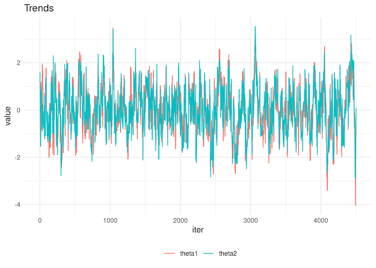
Figure 5
6.4 Select the autocorrelation function below corresponding to the chains in Figure 4 of the previous question.
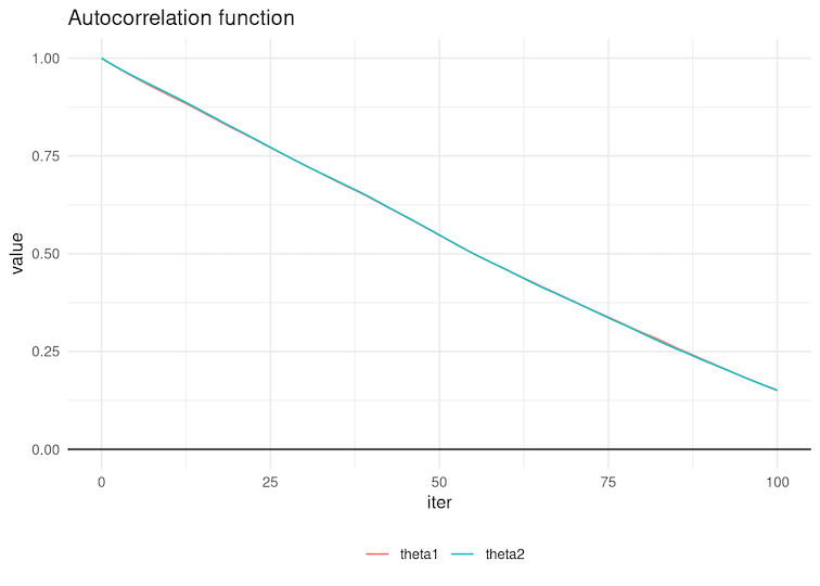
Figure 6
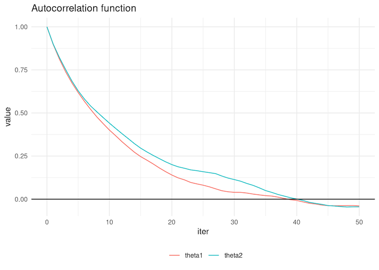
Figure 7
7. Generalised linear model: Bioassay model with Metropolis algorithm
In this exercise, you will implement the Metropolis algorithm. Here you are provided code for a Metropolis algorithm, however, it contains three errors. Your task is to find these errors, correct them and answer the following questions below.
7.1 Lets denote bioassaylp(alpha_propose,
beta_propose, x, y, n) - bioassaylp(alpha_previous, beta_previous, x, y, n)
+ dmvnorm(c(alpha_propose, beta_propose), prior_mean, prior_sigma, TRUE) -
dmvnorm(c(alpha_previous, beta_previous), prior_mean, prior_sigma,
TRUE) as expression 1. How should we correct error 1:
7.2 Lets denote if(runif(1) >
density_ratio(alpha_propose, alpha_previous, beta_propose, beta_previous, x,
y, n)) as expression 2. How should we correct error 2:
7.3: How should we correct error 3:
After you corrected the errors, you may run sampling. Investigate the code in the notebook and answer the questions below.
7.4 How many chains did we run:
7.5 How many draws including warm-up have we obtained for each individual chain
7.6 What is the warm-up length
7.7 After performing sampling, let’s check the convergence of the chains. The next code chunk will produce trace plots. Which one is the correct one:
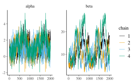
Figure 8
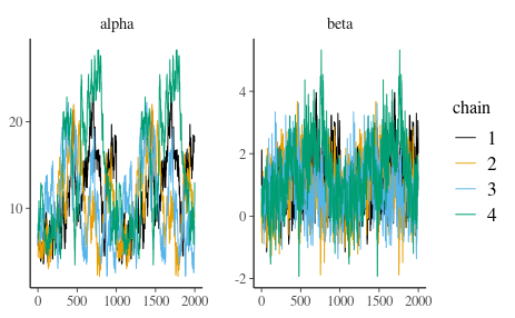
Figure 9
After looking at trace plots, compute Rhat values for both alpha and beta:
7.8 Rhat for alpha
7.9 Rhat for beta
In addition to Rhat, compute ESS for for the mean and 0.25 quantile of alpha and beta:
7.10 ESS mean for alpha
7.11 ESS mean for beta
7.12 ESS q0.25 for alpha
7.13 ESS q0.25 for beta
Let us compare ESS of independent draws and MCMC draws. Use 4000 independent draws from the posterior distribution of the model in the dataset bioassay_posterior in the aaltobda package from Assignment 4.
7.14 ESS mean of alpha for bioassay_posterior
7.15 ESS mean of beta for bioassay_posterior
7.16 ESS q0.25 of alpha for bioassay_posterior
7.17 ESS q0.25 of beta for bioassay_posterior
7.18 Visualise scatter plot of posterior draws. Which one is the correct figure:
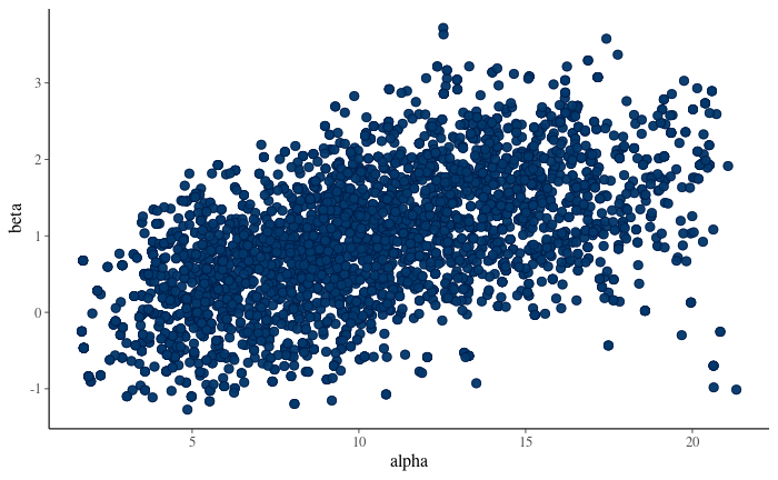
Figure 10
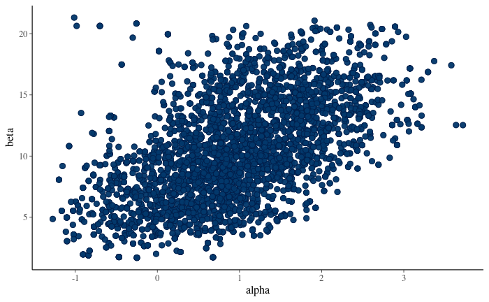
Figure 11